MIST
Magnetosphere, Ionosphere and Solar-Terrestrial
Latest articles
- Analysis of Chorus Wave Power on Burst‐Mode Timescales During the Van Allen Probes Era
- Soft X-Ray Emission from Saturn's Magnetosheath II: Solar Wind Driving
- Which Kelvin-Helmholtz waves grow along the spatially-varying magnetopause flanks and why?
- A new declining phase precursor and an early prediction of cycle 26 maximum
- Short-Term Variability of Jupiter's Satellite Footprints as Spotted by JWST
Latest news
Open Letter Ready For Signatories
Protect MIST Science! Sign the MIST Community Open Letter on the STFC funding cuts!
https://sites.google.com/view/uk-mist-community-open-letter
Statement from MIST Council regarding the STFC Funding Situation
Statement from MIST Council regarding the STFC Funding Situation
MIST Council is deeply concerned by the ongoing STFC funding uncertainty and its impact on our community and beyond.
The current combination of prospective delayed and reduced funding, together with already volatile financial situations at universities across the UK, is placing significant strain on research groups. In some cases, institutions may be unable to support researchers through gaps between projects, increasing precarity across the community and adding significant pressure on early-career researchers.
We are concerned that continued uncertainty risks accelerating a brain drain from the UK, as skilled researchers reconsider their future in a system offering limited stability. The loss of expertise at any career stage would have lasting consequences for UK space science.
What is going on?
For those that are unaware of the situation, it is complex and evolving. We suggest the following sources to get up to speed on the current developments.
https://ras.ac.uk/news-and-press/news/proposed-budget-cuts-catastrophe-uk-astronomy
What are we doing about it?
Behind the scenes, MIST Council is actively engaging with relevant parties to understand the scale of the challenge and to identify constructive ways forward.
- We are seeking seasoned members of the community to join MIST Council on a task force to help develop options and represent the needs of our community. If you would like to be involved, please reach out to us via the MIST Council email (This email address is being protected from spambots. You need JavaScript enabled to view it.) by the end of this week (13th February 2026).
- In addition to the task force, we want to provide an open forum for discussion and collective input among all members of the wider MIST community. We are exploring options and will be in touch as soon as possible with further details.
- We believe in working together in the face of the current challenges and we are collaborating with UKSP and others to strive for a fair and positive outcome for all. We are reaching out to members of the SSAP (Solar System Advisory Panel) to explore the hosting of a community town hall meeting, like the one already being organised by the AAP (Astronomy Advisory Panel), to provide an open forum for discussion and collective input.
What can you do to help?
There are several open letters representing people in various career stages that have been made available to sign. We encourage you to read the relevant letter(s) and to sign them if you support them:
- Fellowship Holders: https://advancedfellows-openletter-stfc.github.io/index.html
- Early Career Researchers: https://ecr-openletter-stfc.github.io/
The Royal Astronomical Society are also urging Fellows to lobby their MPs against the cuts, and have included a template letter that can be used to do so:
https://ras.ac.uk/news-and-press/news/ras-fellows-urged-lobby-against-unprecedented-cuts
MIST Council will continue to advocate for transparency, stability, and funding structures that recognise both the long-term nature of our science and the people who deliver it.
We thank you for your continued support in this period of uncertainty.
Please contact This email address is being protected from spambots. You need JavaScript enabled to view it. if you have further suggestions.
MIST Council
![]()
Announcement of New MIST Council 2025
We are very pleased to announce the following members of the community have been elected to MIST Council:
- Gemma Bower (University of Leicester), MIST Councillor
- Tom Elsden (University of St Andrews), MIST Councillor
- Cameron Patterson (Lancaster University), MIST Councillor
- Fiona Ball (University of Southampton), Student Representative
They will begin their terms in July 2025.
We thank outgoing MIST Council members: Maria Walach, Chiara Lazzeri and Emma Woodfield. Andy Smith will remain on council a little longer as a co-opted member to cover Rosie Johnson's maternity leave.
The current composition of Council can be found on our website (https://www.mist.ac.uk/community/mist-council).
Announcement of New MIST Councillors.
We are very pleased to announce the following members of the community have been elected unopposed to MIST Council:
- Rosie Johnson (Aberystwyth University), MIST Councillor
- Matthew Brown (University of Birmingham), MIST Councillor
- Chiara Lazzeri (MSSL, UCL), Student Representative
Rosie, Matthew, and Chiara will begin their terms in July. This will coincide with Jasmine Kaur Sandhu, Beatriz Sanchez-Cano, and Sophie Maguire outgoing as Councillors.
The current composition of Council can be found on our website, and this will be amended in July to reflect this announcement (https://www.mist.ac.uk/community/mist-council).
Nominations are open for MIST Council
We are very pleased to open nominations for MIST Council. There are three positions available (detailed below), and elected candidates would join Georgios Nicolaou, Andy Smith, Maria-Theresia Walach, and Emma Woodfield on Council. The nomination deadline is Friday 31 May.
Council positions open for nomination
2 x MIST Councillor - a three year term (2024 - 2027). Everyone is eligible.
MIST Student Representative - a one year term (2024 - 2025). Only PhD students are eligible. See below for further details.
About being on MIST Council
If you would like to find out more about being on Council and what it can involve, please feel free to email any of us (email contacts below) with any of your informal enquiries! You can also find out more about MIST activities at mist.ac.uk. Two of our outgoing councillors, Beatriz and Sophie, have summarised their experiences being on MIST Council below.
Beatriz Sanchez-Cano (MIST Councillor):
"Being part of the MIST council for the last 3 years has been a great experience personally and professionally, in which I had the opportunity to know better our community and gain a larger perspective of the matters that are important for the MIST science progress in the UK. During this time, I’ve participated in a number of activities and discussions, such as organising the monthly MIST seminars, Autumn MIST meetings, writing A&G articles, and more importantly, being there to support and advise our colleagues in cases of need together with the wonderful council members. MIST is a vibrant and growing community, and the council is a faithful reflection of it."
Sophie Maguire (MIST Student Representative):
"Being the student representative for MIST council has been an amazing experience. I have been part of organizing conferences, chairing sessions, and writing grant applications based on the feedback MIST has received. From a wider perspective, MIST has helped to grow and support my professional networks which in turn, directly benefits my PhD work as well. I would encourage any PhD student to apply for the role of MIST Student Representative and I would be happy to answer any questions or queries you have about the role."
How to nominate
If you would like to stand for election or you are nominating someone else (with their agreement!) please email This email address is being protected from spambots. You need JavaScript enabled to view it. by Friday 31 May. If there is a surplus of nominations for a role, then an online vote will be carried out with the community. Please include the following details in the nomination:
- Name
- Position (Councillor/Student Rep.)
- Nomination Statement (150 words max including a bit about the nominee and focusing on your reasons for nominating. This will be circulated to the community in the event of a vote.)
MIST Council details
- Sophie Maguire, University of Birmingham, Earth's ionosphere - This email address is being protected from spambots. You need JavaScript enabled to view it.
- Georgios Nicolaou, MSSL, solar wind plasma - This email address is being protected from spambots. You need JavaScript enabled to view it.
- Beatriz Sanchez-Cano, University of Leicester, Mars plasma - This email address is being protected from spambots. You need JavaScript enabled to view it.
- Jasmine Kaur Sandhu, University of Leicester, Earth’s inner magnetosphere - This email address is being protected from spambots. You need JavaScript enabled to view it.
- Andy Smith, Northumbria University, Space Weather - This email address is being protected from spambots. You need JavaScript enabled to view it.
- Maria-Theresia Walach, Lancaster University, Earth’s ionosphere - This email address is being protected from spambots. You need JavaScript enabled to view it.
- Emma Woodfield, British Antarctic Survey, radiation belts - This email address is being protected from spambots. You need JavaScript enabled to view it.
- MIST Council email - This email address is being protected from spambots. You need JavaScript enabled to view it.
Nuggets of MIST science, summarising recent papers from the UK MIST community in a bitesize format.
If you would like to submit a nugget, please fill in the following form: https://forms.gle/Pn3mL73kHLn4VEZ66 and we will arrange a slot for you in the schedule. Nuggets should be 100–300 words long and include a figure/animation. Please get in touch!
If you have any issues with the form, please contact This email address is being protected from spambots. You need JavaScript enabled to view it..
Variation of Geomagnetic Index Empirical Distribution and Burst Statistics Across Successive Solar Cycles
By Aisling Bergin (University of Warwick)
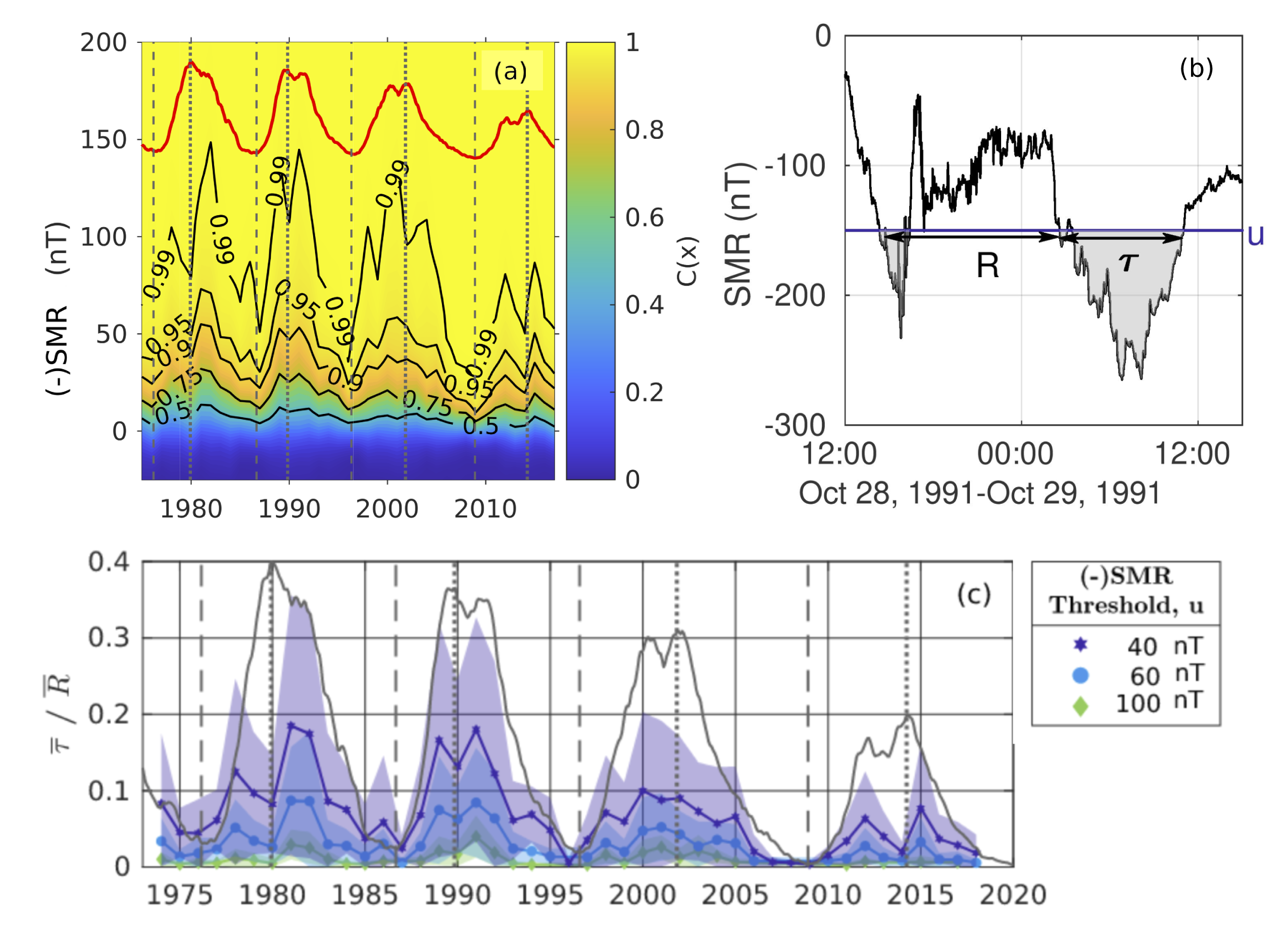
Geomagnetic indices, based on magnetic field observations at the Earth's surface, provide almost continuous monitoring of Earth’s magnetospheric and ionospheric activity. We analyze two geomagnetic index time series, AE and SMR, which track activity in the auroral region and around the Earth's equator, respectively. We show here that quantiles of the index distributions track solar cycle variation over solar cycles 21–24. The question is then how the likelihood of events varies with solar cycle activity.
In this paper, events are defined as bursts or excursions above a threshold which is either (i) a fixed value or (ii) a quantile of the distribution of the observed index values. We study the solar cycle dependence of the distributions of the burst return periods, R, and the burst durations, τ. A result from the theory of level crossings (LC) [1] constrains how , the ratio of the mean burst duration to return period, depends on the underlying empirical distribution of the observed quantity.
Our main results are as follows:
- At fixed value burst thresholds, is peaked in the declining phase for AE annual samples and follows the sunspot number double peak for SMR.
- Bursts are identified in samples at three distinct phases of the solar cycle. At fixed quantile thresholds the distributions of τ and R fall on single empirical curves for each of (i) the AE index at solar minimum, maximum, and declining phase and (ii) the SMR index at solar maximum. This goes beyond the constraint on average from LC theory.
- The tail of the empirical cumulative distribution functions of the observed values of the AE and SMR indices collapse onto common functional forms specific to each index and cycle phase when normalized to the first two moments of their exceedance distributions.
Taken together, these results may combine to offer important constraints in the quantification of overall space weather activity levels.
Please see the paper for full details: Bergin, A., Chapman, S. C., Moloney, N. R., & Watkins, N. W. (2022). Variation of geomagnetic index empirical distribution and burst statistics across successive solar cycles. Journal of Geophysical Research: Space Physics, 127, e2021JA029986. https://doi.org/10.1029/2021JA029986
[1] Lawrance, A., & Kottegoda, N. (1977). Stochastic modelling of riverflow time series. Journal of the Royal Statistical Society: Series A, 140(1), 1–31. https://doi.org/10.2307/2344516
Saturn's Weather‐Driven Aurorae Modulate Oscillations in the Magnetic Field and Radio Emissions
By Nahid Chowdhury (University of Leicester)
Planetary parameters at Saturn have exhibited mysterious time variabilities and periodicities for almost two decades. After the first Voyager measurements of the 1980s led to a determination of a rotation rate for the ringed planet, the advent of the Cassini mission in the 2000s showed that the measured length of a day at Saturn was subject to change. Numerous theories were proposed to explain the time variabilities seen in planetary parameters ranging from the radio emission through to the energies of neutral atoms and these fell into one of two general categories. The first was that a driving mechanism for the observed periodic behaviour would be situated externally to the planet, within the magnetosphere. The second was that a driving mechanism would be situated within the planet’s atmosphere.
Using infrared observations of Saturn’s northern polar auroral H3+ emission taken with Keck-NIRSPEC in 2017, we investigated ion flows in our search for a signature of the twin-vortex mechanism in the planet’s upper atmosphere that was purported to drive the observed periodicities. H3+ is an ion found in the ionosphere of gas giant planets and measurements of its line-of-sight velocity are indicative of the more general motion of constituents in the planet’s atmosphere.
By grouping our spectral data into quadrants of local northern planetary magnetic phase, we set up our experiment to probe the ion flows driven by the planetary period current. This led to the astonishing detection of the proposed ionospheric twin-vortices that are considered to be responsible for the periodicities witnessed throughout Saturn’s planetary and magnetospheric environments. Our observations show that local atmospheric weather effects at Saturn drive the twin-vortex flows while also generating some auroral emissions. This result has far-reaching implications for both other planets in our Solar System and exoplanetary systems.
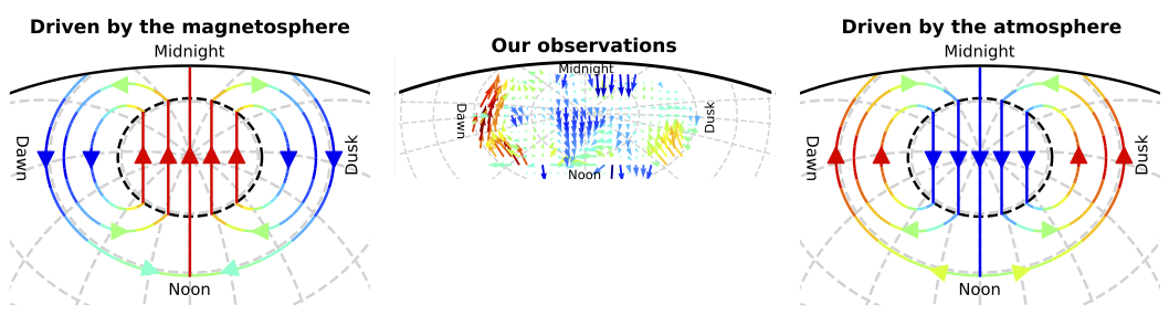
Figure caption: Shown here is an example of the type of winds within the upper atmosphere that are driving the ionosphere to move in the way observed in this new paper. This set of two vortices rotate around the pole of the planet, driving currents within the ionosphere, which then reach out into the surrounding magnetosphere, producing the bright aurora and magnetic field changes observed by Cassini. This weather system was originally proposed by Chris Smith in a paper in Monthly Notices of the Royal Astronomical Society in 2011 (doi:10.1111/j.1365-2966.2010.17602.x) – and it is these modelled flows that we show here.
Please see paper for full details: Chowdhury, M.N., Stallard, T.S., Baines, K.H., Provan, G., Melin, H., Hunt, G.J., Moore, L., O’Donoghue, J., Thomas, E.M., Wang, R. and Miller, S., 2022. Saturn's Weather‐Driven Aurorae Modulate Oscillations in the Magnetic Field and Radio Emissions. Geophysical Research Letters, 49(3), p.e2021GL096492. DOI: https://doi.org/10.1029/2021GL096492.
Modelling the Varying Location of Field Line Resonances During Geomagnetic Storms
By Tom Elsden (University of Glasgow)
Field line resonances (FLRs) are the manifestation of a magnetohydrodynamic (MHD) wave coupling process where energy is transferred from a global to local field-aligned wave. The ‘resonance’ comes from a frequency matching between these waves and being a resonant process, can result in a significant accumulation of energy on a given field line. These waves play an important role in magnetospheric wave-particle interactions, the generation of aurora and can further be used as a seismological tool to remote sense the magnetosphere from ground-based observations.
The location where FLRs occur is intrinsically linked to the current state of the magnetosphere, with the magnetic field structure, plasma density and solar wind driving conditions all being key factors. Given the drastic effect of a geomagnetic storm on the morphology of the magnetosphere, we considered how such changes impact where FLRs form between storm and non-storm times.
We used ground magnetometer data to determine how the fundamental Alfven frequency of field lines varies over the course of a storm on average. These frequencies were then used to infer a plasma density profile to be used in a numerical MHD model to investigate where the FLRs would form under broadband solar wind driving conditions.
Figure 1 shows results from these simulations, displaying the field-aligned current density as an indication of FLRs, mapped from the ionosphere to the equatorial plane to display the radial structure. The left panel is from a simulation modelling the initial phase of a storm, with the right panel modelling the main phase. We show that for an average storm, the FLR moves radially inward by ~1.7RE (compare vertical line locations). This is caused by a decrease in the fundamental Alfven frequency as well as an increase in the global (fast) wave frequency which drives the FLRs.
The important aspect of the results is the overall trend of more Earthward FLR formation during storms. Particularly if extrapolated to more severe storms, this could have an impact on storm-time wave-particle interactions in the radiation belts.
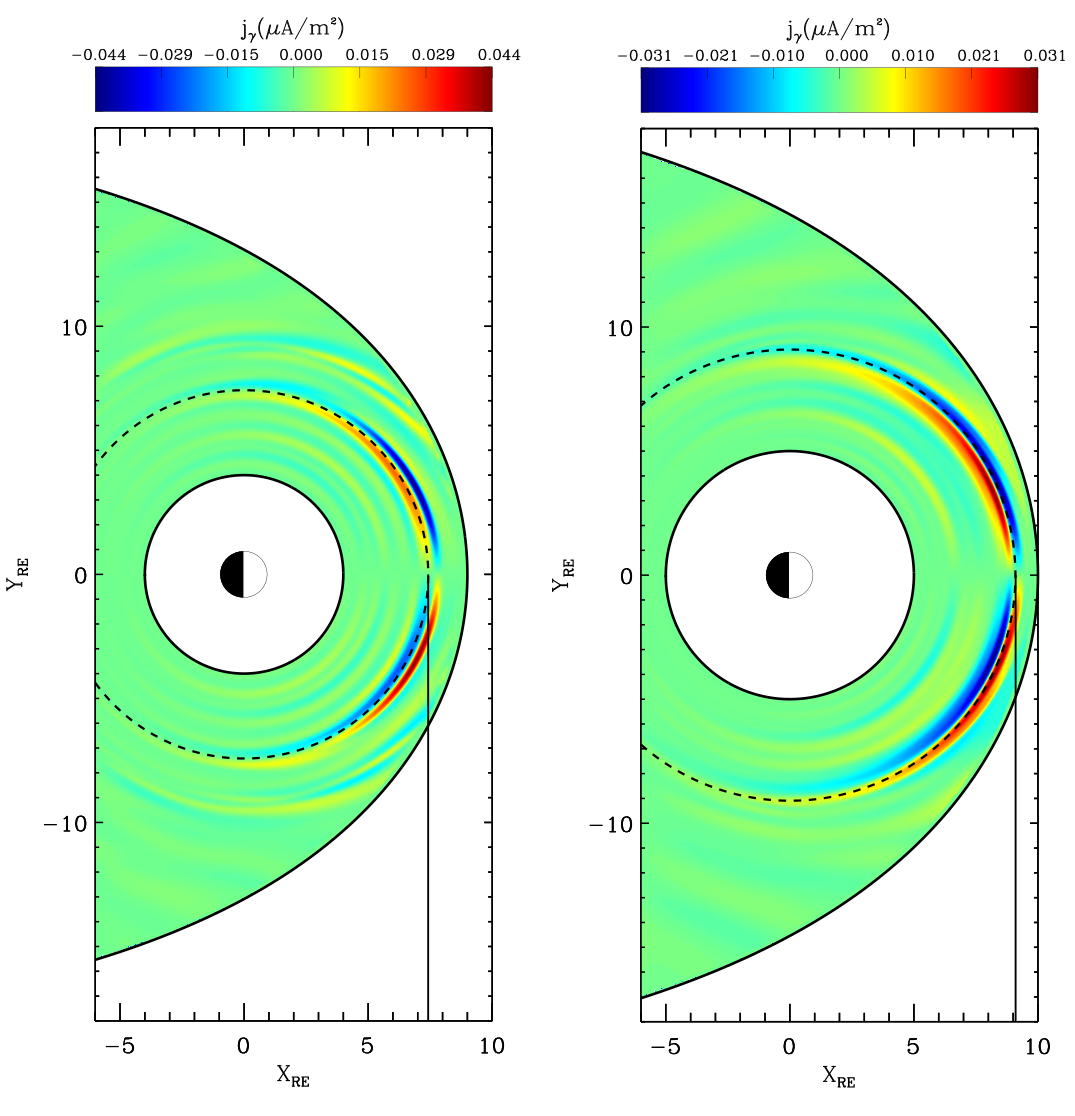
Figure 1 Caption: Colour contours of field-aligned current density from near the ionospheric end of field lines, mapped to the equatorial plane. Left: simulation modelling storm initial phase. Right: simulation modelling storm main phase. Vertical lines indicate field line resonance locations.
Please see paper for full details: Elsden, T., Yeoman, T. K., Wharton, S. J., Rae, I. J., Sandhu, J. K., Walach, M.-T., et al. (2022). Modeling the varying location of field line resonances during geomagnetic storms. Journal of Geophysical Research: Space Physics, 127, e2021JA029804. https://doi.org/10.1029/2021JA029804
Resolving Magnetopause Shadowing Using Multimission Measurements of Phase Space Density
By Frankie Staples (formerly at MSSL UCL, now at UCLA)
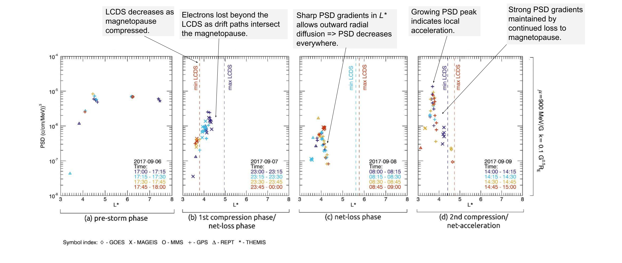
Loss mechanisms act independently or in unison to drive rapid loss of electrons from the radiation belts. Electrons may be lost by precipitation into the Earth’s atmosphere, or through the magnetopause into interplanetary space – a process known as magnetopause shadowing. The mechanisms by which electrons are lost may be identified through changes to electron phase space density (PSD). This method considers the number of particles at given adiabatic coordinates (𝝁, K, and L*), which relate the electron energy, pitch angle, and location in the magnetic field. The characteristics of PSD evolution as a function of L* can be used to identify which loss mechanism is acting. However, the rapid nature of electron flux dropouts make it extremely difficult to resolve PSD dynamics at the necessary timescales to identify the contributions of either loss mechanism.
In this study we used a new multimission dataset of PSD observations from 36 satellites to resolve the dynamics of a magnetopause shadowing induced flux dropout in September 2017. We showed that by using Van Allen Probe data alone, the physical processes causing the dropout could be misinterpreted due to limited time and/or spatial resolution. Using multimission observations provided unprecedented time and spatial resolution necessary to correctly interpret PSD dynamics.
The labelled Figure shows the magnetopause shadowing characteristics identified in PSD observations. Each panel shows PSD as a function of L* for fixed μ = 900 MeV/G and K = 0.1 G0.5RE at 1-hour intervals through phases of the storm. Symbol colours indicate when measurements were taken within the hour period, and dotted lines show the minimum and maximum L* of the last closed drift shell (LCDS) before the magnetopause.
Please see paper for full details:
Staples, F. A., Kellerman, A., Murphy, K. R., Rae, I. J., Sandhu, J. K., & Forsyth, C. (2022). Resolving magnetopause shadowing using multimission measurements of phase space density. Journal of Geophysical Research: Space Physics, 127, e2021JA029298. https://doi.org/10.1029/2021JA029298
Distributions of Birkeland current density observed by AMPERE are heavy‐tailed or long‐tailed
Distributions of Birkeland current density observed by AMPERE are heavy‐tailed or long‐tailed
By John Coxon (Northumbria University)
Electric currents flow above Earth’s surface in the ionosphere; along the magnetopause; across the magnetotail; and in the same region of space as the radiation belts. These currents are all closed through currents flowing along the magnetic field lines in near-Earth space forming one large current circuit; the currents flowing along the field lines are known as field-aligned currents, or as Birkeland currents.
Birkeland currents are, therefore, the currents that communicate impacts from the solar wind (at the magnetopause) and from phenomena such as substorms (in the magnetotail) into the ionosphere, and a key part of the puzzle in understanding phenomena such as ground-based magnetic perturbations such as GICs.
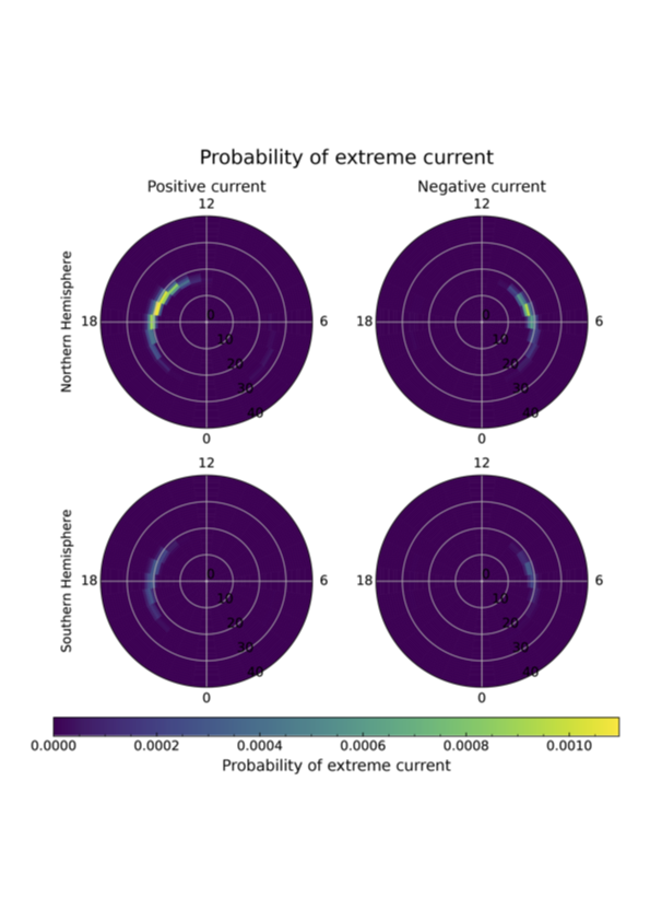
In this paper, we analyse the distributions of the Birkeland current densities measured by a dataset called AMPERE. We find that the distributions are heavy-tailed, which means that they are more likely to display extreme behaviours than if they were distributed normally. We determine that the best model to describe the distributions is a q-exponential model, and we exploit this to find the probability of currents flowing above some given threshold.
We can use this to make maps of the probability of extreme current flows in the Northern and Southern Hemispheres (Figure 1). We can see that the most extreme currents are most likely to be on the dayside of Earth, and at a magnetic colatitude of ~20° (a latitude of ~70°), and we can see that extreme currents are much more likely in the Northern Hemisphere. This has important ramifications for space weather prediction, but also for the physical drivers of the currents; more details are available in the full paper.
Electric currents flow above Earth’s surface in the ionosphere; along the magnetopause; across the magnetotail; and in the same region of space as the radiation belts. These currents are all closed through currents flowing along the magnetic field lines in near-Earth space forming one large current circuit; the currents flowing along the field lines are known as field-aligned currents, or as Birkeland currents.
Birkeland currents are, therefore, the currents that communicate impacts from the solar wind (at the magnetopause) and from phenomena such as substorms (in the magnetotail) into the ionosphere, and a key part of the puzzle in understanding phenomena such as ground-based magnetic perturbations such as GICs.
In this paper, we analyse the distributions of the Birkeland current densities measured by a dataset called AMPERE. We find that the distributions are heavy-tailed, which means that they are more likely to display extreme behaviours than if they were distributed normally. We determine that the best model to describe the distributions is a q-exponential model, and we exploit this to find the probability of currents flowing above some given threshold.
We can use this to make maps of the probability of extreme current flows in the Northern and Southern Hemispheres (Figure 1). We can see that the most extreme currents are most likely to be on the dayside of Earth, and at a magnetic colatitude of ~20° (a latitude of ~70°), and we can see that extreme currents are much more likely in the Northern Hemisphere. This has important ramifications for space weather prediction, but also for the physical drivers of the currents; more details are available in the full paper.