MIST
Magnetosphere, Ionosphere and Solar-Terrestrial
Latest articles
- Analysis of Chorus Wave Power on Burst‐Mode Timescales During the Van Allen Probes Era
- Soft X-Ray Emission from Saturn's Magnetosheath II: Solar Wind Driving
- Which Kelvin-Helmholtz waves grow along the spatially-varying magnetopause flanks and why?
- A new declining phase precursor and an early prediction of cycle 26 maximum
- Short-Term Variability of Jupiter's Satellite Footprints as Spotted by JWST
Latest news
Open Letter Ready For Signatories
Protect MIST Science! Sign the MIST Community Open Letter on the STFC funding cuts!
https://sites.google.com/view/uk-mist-community-open-letter
Statement from MIST Council regarding the STFC Funding Situation
Statement from MIST Council regarding the STFC Funding Situation
MIST Council is deeply concerned by the ongoing STFC funding uncertainty and its impact on our community and beyond.
The current combination of prospective delayed and reduced funding, together with already volatile financial situations at universities across the UK, is placing significant strain on research groups. In some cases, institutions may be unable to support researchers through gaps between projects, increasing precarity across the community and adding significant pressure on early-career researchers.
We are concerned that continued uncertainty risks accelerating a brain drain from the UK, as skilled researchers reconsider their future in a system offering limited stability. The loss of expertise at any career stage would have lasting consequences for UK space science.
What is going on?
For those that are unaware of the situation, it is complex and evolving. We suggest the following sources to get up to speed on the current developments.
https://ras.ac.uk/news-and-press/news/proposed-budget-cuts-catastrophe-uk-astronomy
What are we doing about it?
Behind the scenes, MIST Council is actively engaging with relevant parties to understand the scale of the challenge and to identify constructive ways forward.
- We are seeking seasoned members of the community to join MIST Council on a task force to help develop options and represent the needs of our community. If you would like to be involved, please reach out to us via the MIST Council email (This email address is being protected from spambots. You need JavaScript enabled to view it.) by the end of this week (13th February 2026).
- In addition to the task force, we want to provide an open forum for discussion and collective input among all members of the wider MIST community. We are exploring options and will be in touch as soon as possible with further details.
- We believe in working together in the face of the current challenges and we are collaborating with UKSP and others to strive for a fair and positive outcome for all. We are reaching out to members of the SSAP (Solar System Advisory Panel) to explore the hosting of a community town hall meeting, like the one already being organised by the AAP (Astronomy Advisory Panel), to provide an open forum for discussion and collective input.
What can you do to help?
There are several open letters representing people in various career stages that have been made available to sign. We encourage you to read the relevant letter(s) and to sign them if you support them:
- Fellowship Holders: https://advancedfellows-openletter-stfc.github.io/index.html
- Early Career Researchers: https://ecr-openletter-stfc.github.io/
The Royal Astronomical Society are also urging Fellows to lobby their MPs against the cuts, and have included a template letter that can be used to do so:
https://ras.ac.uk/news-and-press/news/ras-fellows-urged-lobby-against-unprecedented-cuts
MIST Council will continue to advocate for transparency, stability, and funding structures that recognise both the long-term nature of our science and the people who deliver it.
We thank you for your continued support in this period of uncertainty.
Please contact This email address is being protected from spambots. You need JavaScript enabled to view it. if you have further suggestions.
MIST Council
![]()
Announcement of New MIST Council 2025
We are very pleased to announce the following members of the community have been elected to MIST Council:
- Gemma Bower (University of Leicester), MIST Councillor
- Tom Elsden (University of St Andrews), MIST Councillor
- Cameron Patterson (Lancaster University), MIST Councillor
- Fiona Ball (University of Southampton), Student Representative
They will begin their terms in July 2025.
We thank outgoing MIST Council members: Maria Walach, Chiara Lazzeri and Emma Woodfield. Andy Smith will remain on council a little longer as a co-opted member to cover Rosie Johnson's maternity leave.
The current composition of Council can be found on our website (https://www.mist.ac.uk/community/mist-council).
Announcement of New MIST Councillors.
We are very pleased to announce the following members of the community have been elected unopposed to MIST Council:
- Rosie Johnson (Aberystwyth University), MIST Councillor
- Matthew Brown (University of Birmingham), MIST Councillor
- Chiara Lazzeri (MSSL, UCL), Student Representative
Rosie, Matthew, and Chiara will begin their terms in July. This will coincide with Jasmine Kaur Sandhu, Beatriz Sanchez-Cano, and Sophie Maguire outgoing as Councillors.
The current composition of Council can be found on our website, and this will be amended in July to reflect this announcement (https://www.mist.ac.uk/community/mist-council).
Nominations are open for MIST Council
We are very pleased to open nominations for MIST Council. There are three positions available (detailed below), and elected candidates would join Georgios Nicolaou, Andy Smith, Maria-Theresia Walach, and Emma Woodfield on Council. The nomination deadline is Friday 31 May.
Council positions open for nomination
2 x MIST Councillor - a three year term (2024 - 2027). Everyone is eligible.
MIST Student Representative - a one year term (2024 - 2025). Only PhD students are eligible. See below for further details.
About being on MIST Council
If you would like to find out more about being on Council and what it can involve, please feel free to email any of us (email contacts below) with any of your informal enquiries! You can also find out more about MIST activities at mist.ac.uk. Two of our outgoing councillors, Beatriz and Sophie, have summarised their experiences being on MIST Council below.
Beatriz Sanchez-Cano (MIST Councillor):
"Being part of the MIST council for the last 3 years has been a great experience personally and professionally, in which I had the opportunity to know better our community and gain a larger perspective of the matters that are important for the MIST science progress in the UK. During this time, I’ve participated in a number of activities and discussions, such as organising the monthly MIST seminars, Autumn MIST meetings, writing A&G articles, and more importantly, being there to support and advise our colleagues in cases of need together with the wonderful council members. MIST is a vibrant and growing community, and the council is a faithful reflection of it."
Sophie Maguire (MIST Student Representative):
"Being the student representative for MIST council has been an amazing experience. I have been part of organizing conferences, chairing sessions, and writing grant applications based on the feedback MIST has received. From a wider perspective, MIST has helped to grow and support my professional networks which in turn, directly benefits my PhD work as well. I would encourage any PhD student to apply for the role of MIST Student Representative and I would be happy to answer any questions or queries you have about the role."
How to nominate
If you would like to stand for election or you are nominating someone else (with their agreement!) please email This email address is being protected from spambots. You need JavaScript enabled to view it. by Friday 31 May. If there is a surplus of nominations for a role, then an online vote will be carried out with the community. Please include the following details in the nomination:
- Name
- Position (Councillor/Student Rep.)
- Nomination Statement (150 words max including a bit about the nominee and focusing on your reasons for nominating. This will be circulated to the community in the event of a vote.)
MIST Council details
- Sophie Maguire, University of Birmingham, Earth's ionosphere - This email address is being protected from spambots. You need JavaScript enabled to view it.
- Georgios Nicolaou, MSSL, solar wind plasma - This email address is being protected from spambots. You need JavaScript enabled to view it.
- Beatriz Sanchez-Cano, University of Leicester, Mars plasma - This email address is being protected from spambots. You need JavaScript enabled to view it.
- Jasmine Kaur Sandhu, University of Leicester, Earth’s inner magnetosphere - This email address is being protected from spambots. You need JavaScript enabled to view it.
- Andy Smith, Northumbria University, Space Weather - This email address is being protected from spambots. You need JavaScript enabled to view it.
- Maria-Theresia Walach, Lancaster University, Earth’s ionosphere - This email address is being protected from spambots. You need JavaScript enabled to view it.
- Emma Woodfield, British Antarctic Survey, radiation belts - This email address is being protected from spambots. You need JavaScript enabled to view it.
- MIST Council email - This email address is being protected from spambots. You need JavaScript enabled to view it.
Nuggets of MIST science, summarising recent papers from the UK MIST community in a bitesize format.
If you would like to submit a nugget, please fill in the following form: https://forms.gle/Pn3mL73kHLn4VEZ66 and we will arrange a slot for you in the schedule. Nuggets should be 100–300 words long and include a figure/animation. Please get in touch!
If you have any issues with the form, please contact This email address is being protected from spambots. You need JavaScript enabled to view it..
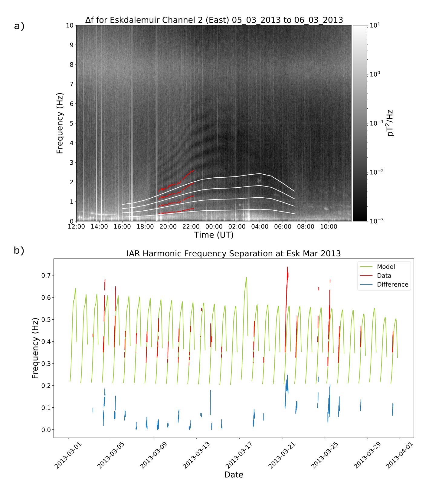
The Harmonic Frequency Separation of Ionospheric Alfvén Resonances at Eskdalemuir
Rosie Hodnett (University of Leicester)
Ionospheric Alfvén resonances (IAR) occur when Alfvén waves are partially reflected at boundaries in the ionosphere where there are large changes in plasma mass density. These boundaries are the bottom of the ionosphere and above the F-Region peak. This sets up a resonance (Belyaev et al., 1990).
IAR have been observed in the induction coil magnetometer data at Eskdalemuir Geophysical Observatory, which is a British Geological Survey site (Beggan & Musur, 2018).
We have modelled the harmonic frequency separation (Δf) of the IAR, by modelling the Alfvén velocity and calculating the time taken for the wave to travel up and down the IAR cavity. We used the International Reference Ionosphere to model the plasma mass density and the International Geomagnetic Reference Field to model the magnetic field strength.
To find the average Δf from the data, we used machine learning to identify the IAR harmonics in spectrograms, and then automatically extracted the frequencies. We used a u-net (Ronneberger et al., 2015) which was developed by Marangio et al. (2020) to detect the IAR.
Figure a) shows the spectrogram for 05/03/2013 – 06/03/2013. The IAR harmonics are visible as bright fringes. The red line lowest in frequency is the average Δf extracted from the data, with subsequent red lines being 2 x Δf, 3 x Δf and 4 x Δf. These are plotted so we can see the Δf following the trends of the harmonics. The lowest white line is the modelled Δf, with higher white lines being higher orders. Generally, the model agrees fairly well with the data. Here, both the data and the model show Δf increasing from dusk to midnight. The data diverges from the model later on, indicating that the model does not accurately capture the ionosphere at this time.
Figure (b) shows the modelled Δf in green, Δf from the data in red and the absolute difference between them in blue, for March 2013. Overall, the data and the model agree well. On 21/03/2013, there is a greater difference between the model and data than other days. Examples like this will be investigated further.
We are now performing further analysis of the 9 year dataset, including a comparison of the data and model to foF2, sunspot number, Sym-H and Kp.
References:
Beggan, C. D., & Musur, M. (2018). Observation of Ionospheric Alfvén Resonances at 1-30 Hz and their Superposition with the Schumann Resonances. Journal of Geophysical Research: Space Physics, 123 (5), 4202–4214. doi: 10.1029/2018ja025264
Belyaev, P., Polyakov, S., Rapoport, V., & Trakhtengerts, V. (1990). The Ionospheric Alfvén Resonator. Journal of Atmospheric and Terrestrial Physics, 52 (9), 781–788. doi: 10.1016/0021-9169(90)90010-k
Marangio, P., Christodoulou, V., Filgueira, R., Rogers, H. F., & Beggan, C. D. (2020). Automatic Detection of Ionospheric Alfvén Resonances in Magnetic Spectrograms using U-Net. Computers amp; Geosciences, 145 , 104598. doi:10.1016/j.cageo.2020.104598
Ronneberger, O., Fischer, P., & Brox, T. (2015). U-Net: Convolutional Networks for Biomedical Image Segmentation. Lecture Notes in Computer Science, 234–241. doi:10.1007/978-3-319-24574-4 287
Acknowledgements:
BGS: www.geomag.bgs.ac.uk/operations/eskdale.html
IRI: www.irimodel.org
IGRF: https://www.ngdc.noaa.gov/IAGA/vmod/igrf.html
Jupiter’s X-Ray and UV Dark Polar Region
By Daisy May and Ben Sipos (St Gilgen’s School)
Jupiter produces powerful ultraviolet (UV) and X-ray aurorae at the planet’s poles. The emissions take on a variety of dynamic structures, particularly in the swirl and active regions (Figure 1). However, the dark polar region (DPR) consistently demonstrates a lack of auroral emissions. 14 simultaneous Chandra X-ray Observatory and Hubble Space Telescope observations of Jupiter’s Northern aurorae (between 2016 and 2019) revealed that no statistically significant X-ray signature is detectable within the DPR.
There were two potential non-DPR sources that might have contributed DPR photons, that needed to be considered. The first source was scattered solar photons. By shifting a region the same shape and size as the observed DPR across non-auroral longitudes of the planet, and scaling the photon counts to the duration of the HST observation, we determined the expected number of scattered photons in the DPR for each observation (0.3 to 1.4 counts depending on the DPR size, distance to Jupiter, and solar activity).
The second source was emissions perceived to have come from within the DPR due to the spatial uncertainty of the X-ray Observatory. To determine the count of such photons, we simulated where photons that were produced from the active and swirl regions would have been detected when passed through the spatial uncertainties applied by the X-ray observatory. After 100,000 simulations for each observation, we determined the count of such falsely detected photons, and found that there is no statistically significant X-ray detection from the DPR for these 14 observations.
The lack of x-rays implies low levels of precipitation by solar wind and energetic magnetospheric ions in the DPR. Therefore, the observations are consistent with the DPR being associated with either: Jupiter’s open field line region and/or the DPR containing different potential drops or an absence of the strong downward currents and/or wave-particle interactions present across the rest of the polar aurorae.
This research project was undertaken with the Orbyts programme which partners scientists with schools to support school student involvement in research and to improve inclusivity in science. This nugget was written by two school students who produced a significant proportion of the work in the associated paper.
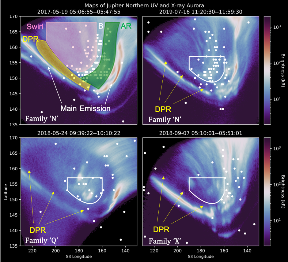
Figure 1: Overlaid simultaneous UV (blue-white-red color map) and X-ray photon (white dots) longitude-latitude maps of Jupiter's North Pole, from the Hubble Space Telescope (HST) and Chandra X-ray Observatory High Resolution Camera (CXO-HRC). Dates and times of the observations (UT) are at the top of each panel. Only UV and X-ray emissions produced during this time window are shown. Jupiter’s main emission is labelled by white arrows, the dark polar region (DPR) is shown in yellow, the Swirl region is shown in pink and the Active Regions (sometimes split into a noon and dusk active region) are shown in Green. The boundary between the active region and swirl region (here labelled with a white “B”) sometimes includes an arc of UV and X-ray emission, as is the case for the two different observations shown in the top two panels here. The other panels highlight three different UV aurora families, as indicated by the white label in the lower left corner of each (Grodent et al. 2018). The white shape overlaid onto each map is consistent across each, and highlights the changing spatial distribution of X-rays for each. For each panel, the location and extent of the DPR are indicated with yellow arrows, showcasing its changing extent from observation-to-observation.
References: Grodent, D., Bonfond, B., Yao, Z., Gérard, J.-C., Radioti, A., Dumont, M., et al. (2018). Jupiter’s aurora observed with HST during Juno orbits 3 to 7. Journal of Geophysical Research: Space Physics, 123(5), 3299– 3319.
Associated Paper: Dunn, W.R., Weigt, D.M., Grodent, D., Yao, Z.H., May, D., Feigelman, K., Sipos, B., Fleming, D., McEntee, S., Bonfond, B. and Gladstone, G.R., 2022. Jupiter’s X‐ray and UV Dark Polar Region. Geophysical Research Letters, p.e2021GL097390.
Data Assimilation and the Solar Wind
By Harriet Turner (University of Reading)
Data assimilation (DA) combines model output and observations to form an optimal estimation of reality. It has led to large improvements in terrestrial weather prediction, reducing the “butterfly effect”, by which small errors in the initial conditions can grow non-linearly and lead to large errors in the subsequent forecast.
DA has been used in three main areas for space weather forecasting: the ionosphere, the photosphere, and, more recently, the solar wind. The first attempts at using DA for solar wind forecasting has shown promise, with a reduction in forecast error (Lang, 2021).
I have been using the Burger Radius Variational Data Assimilation (BRaVDA) scheme (Lang, 2019). This uses output from a coronal model with a computationally efficient solar wind model (HUX; Riley and Lionello, 2011) to map information from in-situ observations at Earth’s orbital radius (215 solar radii), back to the HUX inner boundary at 30 solar radii. The inner boundary conditions are then updated, given the information from the in-situ observations. This update is then run forward in time, again using HUX, to produce a reconstruction of the solar wind. This can then be used for forecasting.
We have three sources of observations: STEREO-A, STEREO-B, and the OMNI dataset for near-Earth space. For the purposes of my work, I am using a simple corotation to produce a forecast. We can compare this forecast against observations from the three sources to assess its performance. Recently, I have been looking at testing the performance of BRaVDA with real time data. Previous experiments have used cleaned-up, science-level data, but real time data would need to be used for an operational DA scheme. Initial results show that using the real time data does not worsen the forecasts significantly and is still an improvement from a 27-day persistence forecast, as shown in Figure 1, which is promising for future implementation of solar wind DA.
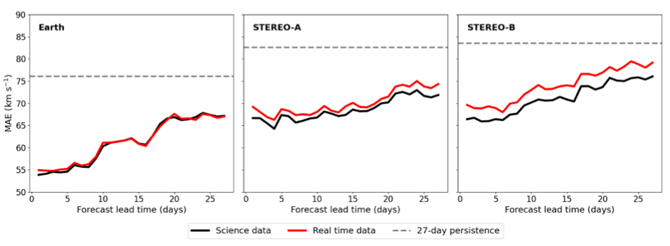
Figure 1: Mean absolute error (MAE) of solar wind forecasts as a function of forecast lead time, for the case where OMNI, STEREO-A and STEREO-B observations are assimilated together. The black line shows the forecast where the science-level data was used and the red line when real time data was used. The dashed grey line shows the average 27-day persistence MAE for the specific spacecraft. The left-hand panel shows the forecast at Earth, the middle panel shows the forecast at STEREO-A and the right-hand panel shows the forecast at STEREO-B. This covers the period from 01/04/2012 to 01/10/2013.
References:
Lang, M., & Owens, M. J. (2019). A Variational Approach to Data Assimilation in the Solar Wind. Space Weather, 17(1), 59 – 83. Doi: 10.1029/2018SW001857.
Lang, M., Witherington, J., Owens, M. J., & Turner, H. (2021). Improving solar wind forecasting using data assimilation. Space Weather, 1 – 23.
Riley, P., & Lionello, R. (2011). Mapping Solar Wind Streams from the Sun to 1 AU: A Comparison of Techniques. Solar Physics, 270(2), 575 – 592. Doi: 10.1007/s11207-001-9766-x.
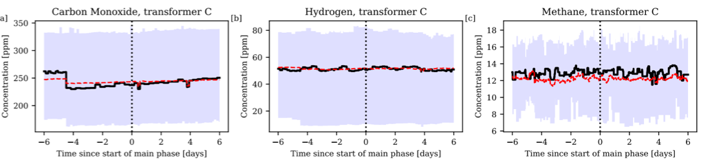
Assessing the Impact of Weak and Moderate Geomagnetic Storms on UK Power Station Transformers
By Zoë Lewis (Imperial College London)
Geomagnetically induced currents (GICs) are known to cause damage to power station transformers, as they can flow through the grounded neutral and generate extra magnetic flux, causing localised heating. This heating can break down the insulation and cooling oil that surrounds the core, so can be measured through small changes in the concentrations of dissolved gases within the oil.
In this work, we analysed dissolved gas data from 13 UK based transformers during geomagnetic storms from 2010-2015. We used a list of storms outlined in [1] and looked for an increase in the levels of carbon monoxide, hydrogen, and methane at the onset of the storm, as well as any correlation between the rate of gas increase and the SYM-H index. We also used the Low Energy Degradation Triangle (LEDT) method [2] as a measure of degradation.
Figure 1 shows the results of a superposed epoch analysis (SEA) for carbon monoxide, methane and hydrogen in one transformer. The epochs are centred on the start of the main phase of each storm, as defined in [1]. There is no systematic increase in the gas concentrations at the storm onset or in the following days. The interquartile range (shaded blue) is also very large owing to the highly variable data.
We conclude that during this period, the transformers studied were unaffected by space weather events. However, it is noted that 2010-2015 lies within a relatively quiet solar cycle, and there were no storms in this period that would be considered large on the scale of the past few decades. Therefore, in future work it would be desirable to expand this study to look at a more geomagnetically active period.
[1] Walach, M. T., & Grocott, A. (2019). SuperDARN Observations During Geomagnetic Storms, Geomagnetically Active Times, and Enhanced Solar Wind Driving. Journal of Geophysical Research: Space Physics, 124 (7), 5828–5847. doi: 10.1029/2019JA026816
[2] Moodley, N., & Gaunt, C. T. (2017). Low Energy Degradation Triangle for power transformer health assessment. IEEE Transactions on Dielectrics and Electrical Insulation, 24 (1), 639–646. doi: 10.1109/TDEI.2016.006042
Please see paper for full details: , , , & (2022). Assessing the impact of weak and moderate geomagnetic storms on UK power station transformers. Space Weather, 20, e2021SW003021. https://doi.org/10.1029/2021SW003021
Transpolar Arcs: Seasonal Dependence Identified by an Automated Detection Algorithm
By Gemma E Bower (University of Leicester)
Transpolar arcs (TPAs) are primarily a northward IMF auroral phenomena. They consist of an arc of auroral emission poleward of the main auroral oval. Their presence suggests that the magnetosphere has a complicated magnetic topology. Currently, TPA formation and evolution have no single explanation that is unanimously agreed upon.
In order to further study the occurrence of TPAs we have developed an automated detection algorithm to determine the occurrence of TPAs in UV images captured by the Defense Meteorological Satellite Program/ Special Sensor Ultraviolet Spectrographic Imager (DMSP/SSUSI) from spacecraft F16, F17, and F18. The detection algorithm identified TPAs as a peak in the average radiance intensity poleward of 12.5° colatitude, in two or more of the wavelengths/bands sensed by SSUSI.
Over 5,000 SSUSI images containing TPAs were identified by the detection algorithm between the years 2010 to 2016. Figure 1a and b shows the seasonal and UT distribution for the F16 TPA images respectively. The occurrence of these TPA images shows a seasonal dependence, with more arcs being visible in the winter hemisphere. There is also an apparent dependence on time-of-day, especially in the southern hemisphere where no TPAs are seen between 23 and 06 UT.
We investigated the effect that the orbital plane of DMSP has on the area of the detection window scanned, as a possible explanation of the dependences in the results of the detection algorithm. Figure 1c and 1d show the results for F16 for seasonal and UT distribution respectively. It can be seen that the orbital plane of DMSP leads to a preferential observation of the northern hemisphere, and the detection algorithm missing TPAs in the southern hemisphere around 01–06 UT. Hence, we conclude that there is no dependence of TPA occurrence on UT. No seasonal bias in the observations is found, indicating that the seasonal dependence of the TPA occurrence is real. We discuss the ramifications of these findings in terms of proposed TPA generation mechanisms.
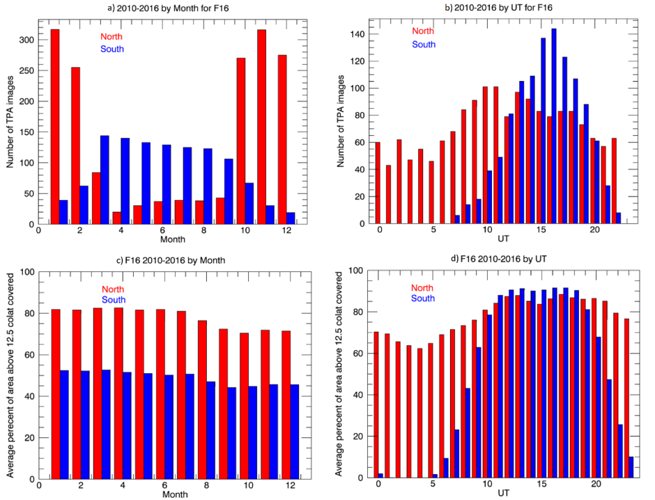
Figure 1: (a-b) Number of transpolar arc (TPA) images identified by F16 between 2010 and 2016. (c-d) Average percent of the detection window poleward of 12.5° colatitude scanned by F16 between 2010 and 2016. (a and c) By month. (b and d) By UT. The northern hemisphere is red and the southern hemisphere is blue
Please see paper for full details: Bower, G. E., Milan, S. E., Paxton, L. J., & Imber, S. M. (2022). Transpolar arcs: Seasonal dependence identified by an automated detection algorithm. Journal of Geophysical Research: Space Physics, 127, e2021JA029743. https://doi.org/10.1029/2021JA029743