MIST
Magnetosphere, Ionosphere and Solar-Terrestrial
Latest articles
- Temporal Variability of Saturn's H2 Dayglow and Northern Aurora Observed by Hisaki and Cassini
- The Jupiter Auroral Ionosphere Code
- Analysis of Chorus Wave Power on Burst‐Mode Timescales During the Van Allen Probes Era
- Soft X-Ray Emission from Saturn's Magnetosheath II: Solar Wind Driving
- Which Kelvin-Helmholtz waves grow along the spatially-varying magnetopause flanks and why?
Latest news
Open Letter Ready For Signatories
Protect MIST Science! Sign the MIST Community Open Letter on the STFC funding cuts!
https://sites.google.com/view/uk-mist-community-open-letter
Statement from MIST Council regarding the STFC Funding Situation
Statement from MIST Council regarding the STFC Funding Situation
MIST Council is deeply concerned by the ongoing STFC funding uncertainty and its impact on our community and beyond.
The current combination of prospective delayed and reduced funding, together with already volatile financial situations at universities across the UK, is placing significant strain on research groups. In some cases, institutions may be unable to support researchers through gaps between projects, increasing precarity across the community and adding significant pressure on early-career researchers.
We are concerned that continued uncertainty risks accelerating a brain drain from the UK, as skilled researchers reconsider their future in a system offering limited stability. The loss of expertise at any career stage would have lasting consequences for UK space science.
What is going on?
For those that are unaware of the situation, it is complex and evolving. We suggest the following sources to get up to speed on the current developments.
https://ras.ac.uk/news-and-press/news/proposed-budget-cuts-catastrophe-uk-astronomy
What are we doing about it?
Behind the scenes, MIST Council is actively engaging with relevant parties to understand the scale of the challenge and to identify constructive ways forward.
- We are seeking seasoned members of the community to join MIST Council on a task force to help develop options and represent the needs of our community. If you would like to be involved, please reach out to us via the MIST Council email (This email address is being protected from spambots. You need JavaScript enabled to view it.) by the end of this week (13th February 2026).
- In addition to the task force, we want to provide an open forum for discussion and collective input among all members of the wider MIST community. We are exploring options and will be in touch as soon as possible with further details.
- We believe in working together in the face of the current challenges and we are collaborating with UKSP and others to strive for a fair and positive outcome for all. We are reaching out to members of the SSAP (Solar System Advisory Panel) to explore the hosting of a community town hall meeting, like the one already being organised by the AAP (Astronomy Advisory Panel), to provide an open forum for discussion and collective input.
What can you do to help?
There are several open letters representing people in various career stages that have been made available to sign. We encourage you to read the relevant letter(s) and to sign them if you support them:
- Fellowship Holders: https://advancedfellows-openletter-stfc.github.io/index.html
- Early Career Researchers: https://ecr-openletter-stfc.github.io/
The Royal Astronomical Society are also urging Fellows to lobby their MPs against the cuts, and have included a template letter that can be used to do so:
https://ras.ac.uk/news-and-press/news/ras-fellows-urged-lobby-against-unprecedented-cuts
MIST Council will continue to advocate for transparency, stability, and funding structures that recognise both the long-term nature of our science and the people who deliver it.
We thank you for your continued support in this period of uncertainty.
Please contact This email address is being protected from spambots. You need JavaScript enabled to view it. if you have further suggestions.
MIST Council
![]()
Announcement of New MIST Council 2025
We are very pleased to announce the following members of the community have been elected to MIST Council:
- Gemma Bower (University of Leicester), MIST Councillor
- Tom Elsden (University of St Andrews), MIST Councillor
- Cameron Patterson (Lancaster University), MIST Councillor
- Fiona Ball (University of Southampton), Student Representative
They will begin their terms in July 2025.
We thank outgoing MIST Council members: Maria Walach, Chiara Lazzeri and Emma Woodfield. Andy Smith will remain on council a little longer as a co-opted member to cover Rosie Johnson's maternity leave.
The current composition of Council can be found on our website (https://www.mist.ac.uk/community/mist-council).
Announcement of New MIST Councillors.
We are very pleased to announce the following members of the community have been elected unopposed to MIST Council:
- Rosie Johnson (Aberystwyth University), MIST Councillor
- Matthew Brown (University of Birmingham), MIST Councillor
- Chiara Lazzeri (MSSL, UCL), Student Representative
Rosie, Matthew, and Chiara will begin their terms in July. This will coincide with Jasmine Kaur Sandhu, Beatriz Sanchez-Cano, and Sophie Maguire outgoing as Councillors.
The current composition of Council can be found on our website, and this will be amended in July to reflect this announcement (https://www.mist.ac.uk/community/mist-council).
Nominations are open for MIST Council
We are very pleased to open nominations for MIST Council. There are three positions available (detailed below), and elected candidates would join Georgios Nicolaou, Andy Smith, Maria-Theresia Walach, and Emma Woodfield on Council. The nomination deadline is Friday 31 May.
Council positions open for nomination
2 x MIST Councillor - a three year term (2024 - 2027). Everyone is eligible.
MIST Student Representative - a one year term (2024 - 2025). Only PhD students are eligible. See below for further details.
About being on MIST Council
If you would like to find out more about being on Council and what it can involve, please feel free to email any of us (email contacts below) with any of your informal enquiries! You can also find out more about MIST activities at mist.ac.uk. Two of our outgoing councillors, Beatriz and Sophie, have summarised their experiences being on MIST Council below.
Beatriz Sanchez-Cano (MIST Councillor):
"Being part of the MIST council for the last 3 years has been a great experience personally and professionally, in which I had the opportunity to know better our community and gain a larger perspective of the matters that are important for the MIST science progress in the UK. During this time, I’ve participated in a number of activities and discussions, such as organising the monthly MIST seminars, Autumn MIST meetings, writing A&G articles, and more importantly, being there to support and advise our colleagues in cases of need together with the wonderful council members. MIST is a vibrant and growing community, and the council is a faithful reflection of it."
Sophie Maguire (MIST Student Representative):
"Being the student representative for MIST council has been an amazing experience. I have been part of organizing conferences, chairing sessions, and writing grant applications based on the feedback MIST has received. From a wider perspective, MIST has helped to grow and support my professional networks which in turn, directly benefits my PhD work as well. I would encourage any PhD student to apply for the role of MIST Student Representative and I would be happy to answer any questions or queries you have about the role."
How to nominate
If you would like to stand for election or you are nominating someone else (with their agreement!) please email This email address is being protected from spambots. You need JavaScript enabled to view it. by Friday 31 May. If there is a surplus of nominations for a role, then an online vote will be carried out with the community. Please include the following details in the nomination:
- Name
- Position (Councillor/Student Rep.)
- Nomination Statement (150 words max including a bit about the nominee and focusing on your reasons for nominating. This will be circulated to the community in the event of a vote.)
MIST Council details
- Sophie Maguire, University of Birmingham, Earth's ionosphere - This email address is being protected from spambots. You need JavaScript enabled to view it.
- Georgios Nicolaou, MSSL, solar wind plasma - This email address is being protected from spambots. You need JavaScript enabled to view it.
- Beatriz Sanchez-Cano, University of Leicester, Mars plasma - This email address is being protected from spambots. You need JavaScript enabled to view it.
- Jasmine Kaur Sandhu, University of Leicester, Earth’s inner magnetosphere - This email address is being protected from spambots. You need JavaScript enabled to view it.
- Andy Smith, Northumbria University, Space Weather - This email address is being protected from spambots. You need JavaScript enabled to view it.
- Maria-Theresia Walach, Lancaster University, Earth’s ionosphere - This email address is being protected from spambots. You need JavaScript enabled to view it.
- Emma Woodfield, British Antarctic Survey, radiation belts - This email address is being protected from spambots. You need JavaScript enabled to view it.
- MIST Council email - This email address is being protected from spambots. You need JavaScript enabled to view it.
Nuggets of MIST science, summarising recent papers from the UK MIST community in a bitesize format.
If you would like to submit a nugget, please fill in the following form: https://forms.gle/Pn3mL73kHLn4VEZ66 and we will arrange a slot for you in the schedule. Nuggets should be 100–300 words long and include a figure/animation. Please get in touch!
If you have any issues with the form, please contact This email address is being protected from spambots. You need JavaScript enabled to view it..
LOFAR Observations of sub-structure within a Travelling Ionospheric Disturbance at mid-latitude
By Gareth Dorrian (Space Environment & Radio Engineering, University of Birmingham)
Travelling ionospheric disturbances (TID) are ubiquitous wave-like propagations in the Earth’s ionosphere and are the ionospheric counterpart of neutral atmospheric gravity waves (AGW). AGW can be driven by numerous sources from both the terrestrial and space weather domain such as sunrise, auroral sub-storms, volcanic eruptions, or thunderstorms. Terrestrial drivers from the lower atmosphere are coupled to the thermosphere by upwards propagation of AGW (Hines, 1960).
We study the ionosphere using LOFAR observations of trans-ionospheric radio propagation from compact natural radio sources. This is advantageous as, unlike most artificial satellites, natural radio sources are inherently broadband emitters and LOFAR is a broadband receiver with high frequency and time resolution. The behaviour of radio scattering through the ionosphere can thus be observed simultaneously across many frequencies.
Observations using the LOw Frequency ARray (LOFAR: van Haarlem et al., 2013) of trans-ionospheric radio propagation through a TID over the UK were made on 7 January 2019 (Figure 1). In LOFAR data, ionospheric variability manifests as rapid changes in the received signal from the radio source. Using this technique, internal sub-structure within the TID were clearly identified with dominant modes of oscillation on timescales of ~300s. At the observing geometries used these oscillations equated to sub-structure scale sizes of ~20 km. Contemporary GNSS and ionosonde data were used to provide the global parameters of the TID. At the observation frequencies used (25-65 MHz) the Fresnel scale is between 3-4 km; consequently the majority of the scattering features observed were lens-like refractions, rather than diffractive scintillation. Geomagnetic conditions at this time were very quiet, suggesting a terrestrial driver.
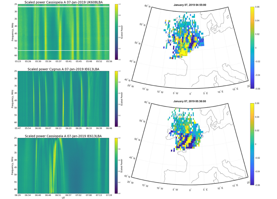
Figure 1: Left panels: LOFAR dynamic spectra from UK and Irish stations showing rapid variations in received signal power across the full observing band, caused by passage of TID internal substructure across raypath. Right panels: GNSS plasma anomaly maps from the observing period with the wave-like form of the TID clearly visible over the UK.
Original article for further details:
Dorrian, G., Fallows, R., Wood, A., Themens, D. R., Boyde, B., Krankowski, A., et al. (2023). LOFAR observations of substructure within a travelling ionospheric disturbance at mid-latitude. Space Weather, 21, e2022SW003198. https://doi.org/10.1029/2022SW003198
References:
van Haarlem, M. P., Wise, M. W., Gunst, A. W., Heald, G., McKean, J. P., Hessels, J. W. T., et al. (2013). LOFAR: Low-frequency-array. Astronomy and Astrophysics, 556, A2. https://doi.org/10.1051/0004-6361/201220873
Hines, C. O. (1960). Internal atmospheric gravity waves at ionospheric heights. Canadian Journal of Physics, 38(11), 1441– 1481. https://doi.org/10.1139/p60-150
Fine‐Scale Electric Fields and Joule Heating From Observations of the Aurora
By Patrik Krcelic (University of Southampton)
Optical measurements from three selected wavelengths have been combined with modelling of emissions from an auroral arc to estimate the magnitude and direction of small-scale electric fields on either side of an auroral arc for an event at 22:47:45 UT on 21 December 2014. The temporal resolution of the estimates is 0.1 s, which is much higher resolution than measurements from Super Dual Auroral Radar Network (SuperDARN) in the same region, with which we compare our estimates. The obtained electric fields have peak value of 88 ± 16 mV/m on the northern side of the arc and peak value of 66 ± 21 mV/m on the southern side of the arc. Additionally, we have used the Scanning Doppler Imager instrument to measure the neutral wind during the event in order to calculate the height integrated Joule heating. Joule heating obtained from small scale electric fields gives much larger values than that obtained from SuperDARN data. Results are briefly shown in the movie below, where the top two panels depict an observed and modelled auroral arc analyzed in current syudy, and the bottom plot depicts the evolution of Joule heating in time on each side of the auroral arc compared with the SuperDARN estimate. Our optical method for estimating electric fields, and consequently the Joule heating using ASK, has proven to be very valuable in understanding the local heating effects in the vicinity of auroral activity. Such high spatial and temporal resolution electric fields may play an important role in the dynamics of the magnetosphere-ionosphere-thermosphere system.
Original article for further detail:
Krcelic, P., Fear, R. C., Whiter, D., Lanchester, B., Aruliah, A. L., Lester, M., & Paxton, L. (2023). Fine-scale electric fields and Joule heating from observations of the aurora. Journal of Geophysical Research: Space Physics, 128, e2022JA030628. https://doi.org/10.1029/2022JA030628
Modeling the Time-Dependent Magnetic Fields That BepiColombo Will Use to Probe Down Into Mercury's Mantle
By Sophia Zomerdijk-Russell (Imperial College London)
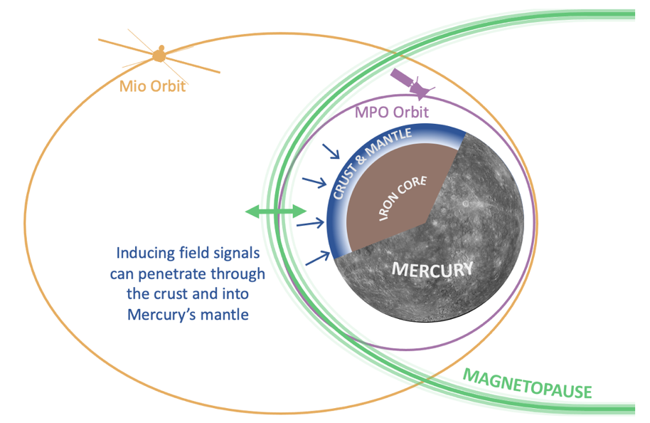
The interior structure of a magnetised planet can be determined by using electromagnetic induction processes that results from solar-wind-driven magnetopause variability. To determine a profile of conductivity through depth within a planet, a broad spectrum of inducing fields is needed, as each discrete frequency will probe to a certain depth.
In preparation for the arrival of BepiColombo at Mercury in 2025, we have identified the opportunity to use Helios data to assess how solar wind ram pressure forcing can drive magnetopause variability at Mercury, as Helios took measurements during a similar phase of the Solar Cycle that BepiColombo is expected to see on its arrival. We find that Mercury’s magnetosphere is bombarded by a highly variable and unpredictable solar wind with a broad range of frequency signals and that the inducing field generated in response to the variable solar wind ram pressure is non-uniform across the planet’s surface.
A solar wind ram pressure time series from Helios measurements and the KT17 Hermean magnetospheric field model (Korth et al., 2017) were then used to generate a ram pressure driven inducing field spectra at two points on Mercury’s surface. In power spectra of these example inducing field spectra, frequency signals were found to peak between ~5.510-5 and 1.510-2 Hz. Heyner et al. (2021) determined that signals with these frequencies should penetrate into Mercury’s crust and mantle.
Particular orbital configurations of the BepiColombo mission will have MPO inside Mercury’s magnetosphere and Mio measuring the upstream solar wind, see Figure 1. Therefore, the dual spacecraft nature of the BepiColombo mission will be well suited to investigate Mercury’s magnetosphere’s response to external solar wind variability and allow a conductivity profile through to the mantle to be derived from observations of solar wind driven inducing field spectra with timescales seen in this work.
Original article for further detail:
, , , & (2023). Modeling the time-dependent magnetic fields that BepiColombo will use to probe down into Mercury's mantle. Geophysical Research Letters, 50, e2022GL101607. https://doi.org/10.1029/2022GL101607
References:
Heyner, D., Auster, H.-U., Fornaçon, K.-H., Carr, C., Richter, I., Mieth, J. Z. D., Kolhey, P., Exner, W., Motschmann, U., Baumjohann, W., Matsuoka, A., Magnes, W., Berghofer, G., Fischer, D., Plaschke, F., Nakamura, R., Narita, Y., Delva, M., Volwerk, M., … Glassmeier, K.-H. (2021). The BepiColombo Planetary Magnetometer MPO-MAG: What Can We Learn from the Hermean Magnetic Field? Space Science Reviews, 217(4), 52. https://doi.org/10.1007/s11214-021-00822-x
Korth, H., Johnson, C. L., Philpott, L., Tsyganenko, N. A., & Anderson, B. J. (2017). A Dynamic Model of Mercury’s Magnetospheric Magnetic Field. Geophysical Research Letters, 44(20), 10,147-10,154. https://doi.org/10.1002/2017GL074699
Variations in Observations of Geosynchronous Magnetopause and Last Closed Drift Shell Crossings With Magnetic Local Time
By Tom Daggitt (British Antarctic Survey, University of Cambridge)
Geostationary satellites may cross the magnetopause during highly active times when it can be compressed inside geostationary orbit. At this time the satellite will switch from observing Earth’s magnetic field to the interplanetary magnetic field, which is usually opposing Earth’s field during compressions. The satellite will observe a drop in electron flux as it goes from measuring trapped electrons in Earth’s radiation belts to electrons in the interplanetary medium.
We compare observations from the GOES-13 and GOES-15 satellites during geomagnetic storms. We attempt to predict magnetopause crossings using models of the last closed drift shell (LCDS), the outermost stable orbit for an electron trapped in Earth’s magnetic field. The LCDS is modelled as the largest L* value that calculated by the IRBEM magnetic field modelling library (Boscher et al., 2013), using a method derived from Albert et al. (2018).
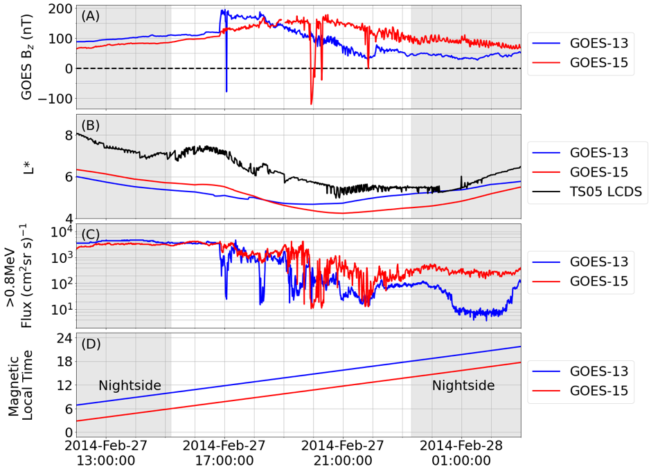
Figure 1(A) shows the Bz component of the field measured by the GOES magnetometers, demonstrating independent magnetopause crossings when the Bz component is negative. Each satellite only sees a magnetopause crossing when it is nearer local noon.
1(B) shows the satellite L* and the LCDS derived from the TS05 field model (Tsyganenko & Sitnov, 2005). Neither satellite crosses the LCDS during their magnetopause crossings, showing that brief crossings cannot be predicted with this method.
1(C) shows the >0.8MeV flux measured by the GOES satellites, showing rapid decreases in the measured flux associated with each magnetopause crossing. GOES-13 also shows a large decrease in flux as it moves into the nightside, likely due to distortion in the magnetotail.
The difference in the observed flux profiles demonstrates that choice of satellite may have a large effect when using satellite data to drive radiation belt models. Data from multiple satellites should be used to ensure constant measurements of the trapped flux on the dayside when driving radiation belt models.
References:
Boscher, D., Bourdarie, S., O’Brien, P., & Guild, T. (2013). Irbem library v4.3, 2004-2008. https://spacepy.github.io/irbempy.html.
Albert, J. M., Selesnick, R., Morley, S. K., Henderson, M. G., & Kellerman, A. (2018). Calculation of last closed drift shells for the 2013 gem radiation belt challenge events. Journal of Geophysical Research: Space Physics, 123(11), 9597– 9611. https://doi.org/10.1029/2018JA025991
Tsyganenko, N., & Sitnov, M. (2005). Modeling the dynamics of the inner magnetosphere during strong geomagnetic storms. Journal of Geophysical Research, 110(A3), A03208. https://doi.org/10.1029/2004JA010798
Associated Paper:
Daggitt, T. A., Horne, R. B., Glauert, S. A., Del Zanna, G., & Freeman, M. P. (2022). Variations in observations of geosynchronous magnetopause and last closed drift shell crossings with magnetic local time. Space Weather, 20, e2022SW003105. https://doi.org/10.1029/2022SW003105
An inner boundary condition for solar wind models based on coronal density
By Kaine Bunting (Aberystwyth University)
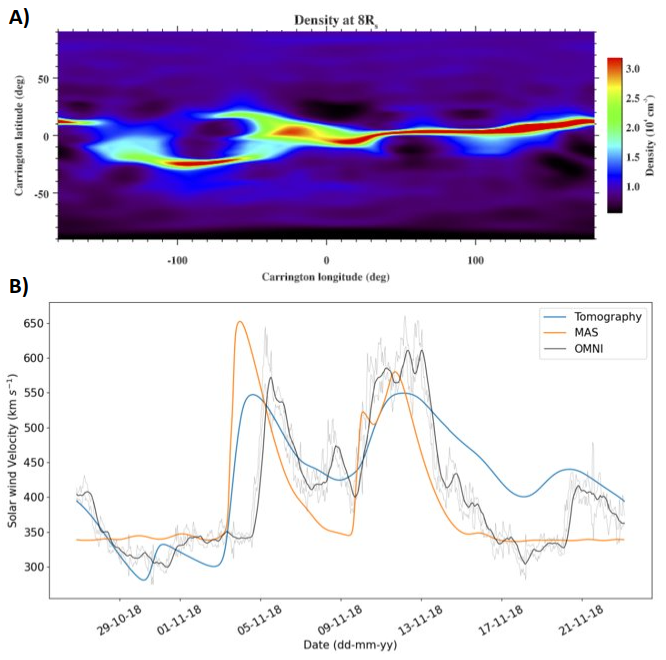
Tomography is used to gain the 3D plasma density of the solar corona (between 4-8Rs) using white light coronagraph observations (Morgan and Cook 2019). In this work, we use the density at 8Rs (e.g. figure 1a) to estimate velocity, providing an inner boundary condition for a heliospheric solar wind model. The results show that tomography can provide a valid (or improved) alternative to traditional photospheric-based magnetic models.
A simple inverse linear relationship converts densities to velocities. Extracted from Earth's latitude, the velocities form an inner boundary condition for the Time-dependent Heliospheric Upwind Extrapolation (HUXt) model (Owens et al. 2020). The model is then simulated for one Carrington rotation (CR), giving predicted velocities at Earth. The modelled velocities are compared to OMNI in-situ data, and the efficiency of HUXt allows an iterative fitting method optimises the parameters of the density-velocity conversion model by minimising a ‘distance’ metric using Dynamic Time Warping (DTW, Samara et al. 2022).
Figure 1 b) compares the output of HUXt based on Tomography-HUXt and MAS inner boundaries (Linker et al. 1999), where the MAS velocities have been optimised similarly to the tomography velocities for CR2210 (Nov 2018). Tomography-HUXt model outperforms the MAS-HUXt model: tomography-HUXt gives a MAE of 47.9 km s-1 compared to the 53.58 km s-1 of the MAS-HUXt model, and a higher Pearson correlation coefficient of 0.74 compared to that of MAS-HUXt (0.56). This work shows that inner boundary conditions derived using tomography are a valid alternative to magnetic models such as MAS.
Our current work investigates a more advanced relationship between coronal densities and velocities, and provides improved solar wind predictions over a whole solar cycle. This scheme is implemented as part of the SWEEP software suite for the UK Met Office's space weather forecasting capabilities from 2023 onwards.
References:
Linker, J. A., Z. Miki ́c, D. A. Biesecker, R. J. Forsyth, S. E. Gibson, et al. 1999. Magnetohydrodynamic modeling of the solar corona during Whole Sun Month. Journal of Geophysical Research: Space Physics, 104. 10.1029/1998ja900159.
Morgan, H., and A. C. Cook, 2020. The Width, Density, and Outflow of Solar Coronal Streamers. The Astrophysical Journal, 893(1), 57. 10.3847/1538-4357/ab7e32
Owens, M. J., M. Lang, L. Barnard, P. Riley, M. Ben-Nun, et al. 2020. A Computationally Efficient, Time-Dependent Model of the Solar Wind for Use as a Surrogate to Three-Dimensional Numerical Magnetohydrodynamic Simulations. Solar Physics. 10.1007/s11207-020-01605-3
Samara, E., B. Laperre, R. Kieokaew, M. Temmer, C. Verbeke, et al. 2022. Dynamic Time Warping as a Means of Assessing Solar Wind Time Series. The Astrophysical Journal, 927(2), 187. 10.3847/1538-4357/ac4af6