MIST
Magnetosphere, Ionosphere and Solar-Terrestrial
Latest articles
- Temporal Variability of Saturn's H2 Dayglow and Northern Aurora Observed by Hisaki and Cassini
- The Jupiter Auroral Ionosphere Code
- Analysis of Chorus Wave Power on Burst‐Mode Timescales During the Van Allen Probes Era
- Soft X-Ray Emission from Saturn's Magnetosheath II: Solar Wind Driving
- Which Kelvin-Helmholtz waves grow along the spatially-varying magnetopause flanks and why?
Latest news
Open Letter Ready For Signatories
Protect MIST Science! Sign the MIST Community Open Letter on the STFC funding cuts!
https://sites.google.com/view/uk-mist-community-open-letter
Statement from MIST Council regarding the STFC Funding Situation
Statement from MIST Council regarding the STFC Funding Situation
MIST Council is deeply concerned by the ongoing STFC funding uncertainty and its impact on our community and beyond.
The current combination of prospective delayed and reduced funding, together with already volatile financial situations at universities across the UK, is placing significant strain on research groups. In some cases, institutions may be unable to support researchers through gaps between projects, increasing precarity across the community and adding significant pressure on early-career researchers.
We are concerned that continued uncertainty risks accelerating a brain drain from the UK, as skilled researchers reconsider their future in a system offering limited stability. The loss of expertise at any career stage would have lasting consequences for UK space science.
What is going on?
For those that are unaware of the situation, it is complex and evolving. We suggest the following sources to get up to speed on the current developments.
https://ras.ac.uk/news-and-press/news/proposed-budget-cuts-catastrophe-uk-astronomy
What are we doing about it?
Behind the scenes, MIST Council is actively engaging with relevant parties to understand the scale of the challenge and to identify constructive ways forward.
- We are seeking seasoned members of the community to join MIST Council on a task force to help develop options and represent the needs of our community. If you would like to be involved, please reach out to us via the MIST Council email (This email address is being protected from spambots. You need JavaScript enabled to view it.) by the end of this week (13th February 2026).
- In addition to the task force, we want to provide an open forum for discussion and collective input among all members of the wider MIST community. We are exploring options and will be in touch as soon as possible with further details.
- We believe in working together in the face of the current challenges and we are collaborating with UKSP and others to strive for a fair and positive outcome for all. We are reaching out to members of the SSAP (Solar System Advisory Panel) to explore the hosting of a community town hall meeting, like the one already being organised by the AAP (Astronomy Advisory Panel), to provide an open forum for discussion and collective input.
What can you do to help?
There are several open letters representing people in various career stages that have been made available to sign. We encourage you to read the relevant letter(s) and to sign them if you support them:
- Fellowship Holders: https://advancedfellows-openletter-stfc.github.io/index.html
- Early Career Researchers: https://ecr-openletter-stfc.github.io/
The Royal Astronomical Society are also urging Fellows to lobby their MPs against the cuts, and have included a template letter that can be used to do so:
https://ras.ac.uk/news-and-press/news/ras-fellows-urged-lobby-against-unprecedented-cuts
MIST Council will continue to advocate for transparency, stability, and funding structures that recognise both the long-term nature of our science and the people who deliver it.
We thank you for your continued support in this period of uncertainty.
Please contact This email address is being protected from spambots. You need JavaScript enabled to view it. if you have further suggestions.
MIST Council
![]()
Announcement of New MIST Council 2025
We are very pleased to announce the following members of the community have been elected to MIST Council:
- Gemma Bower (University of Leicester), MIST Councillor
- Tom Elsden (University of St Andrews), MIST Councillor
- Cameron Patterson (Lancaster University), MIST Councillor
- Fiona Ball (University of Southampton), Student Representative
They will begin their terms in July 2025.
We thank outgoing MIST Council members: Maria Walach, Chiara Lazzeri and Emma Woodfield. Andy Smith will remain on council a little longer as a co-opted member to cover Rosie Johnson's maternity leave.
The current composition of Council can be found on our website (https://www.mist.ac.uk/community/mist-council).
Announcement of New MIST Councillors.
We are very pleased to announce the following members of the community have been elected unopposed to MIST Council:
- Rosie Johnson (Aberystwyth University), MIST Councillor
- Matthew Brown (University of Birmingham), MIST Councillor
- Chiara Lazzeri (MSSL, UCL), Student Representative
Rosie, Matthew, and Chiara will begin their terms in July. This will coincide with Jasmine Kaur Sandhu, Beatriz Sanchez-Cano, and Sophie Maguire outgoing as Councillors.
The current composition of Council can be found on our website, and this will be amended in July to reflect this announcement (https://www.mist.ac.uk/community/mist-council).
Nominations are open for MIST Council
We are very pleased to open nominations for MIST Council. There are three positions available (detailed below), and elected candidates would join Georgios Nicolaou, Andy Smith, Maria-Theresia Walach, and Emma Woodfield on Council. The nomination deadline is Friday 31 May.
Council positions open for nomination
2 x MIST Councillor - a three year term (2024 - 2027). Everyone is eligible.
MIST Student Representative - a one year term (2024 - 2025). Only PhD students are eligible. See below for further details.
About being on MIST Council
If you would like to find out more about being on Council and what it can involve, please feel free to email any of us (email contacts below) with any of your informal enquiries! You can also find out more about MIST activities at mist.ac.uk. Two of our outgoing councillors, Beatriz and Sophie, have summarised their experiences being on MIST Council below.
Beatriz Sanchez-Cano (MIST Councillor):
"Being part of the MIST council for the last 3 years has been a great experience personally and professionally, in which I had the opportunity to know better our community and gain a larger perspective of the matters that are important for the MIST science progress in the UK. During this time, I’ve participated in a number of activities and discussions, such as organising the monthly MIST seminars, Autumn MIST meetings, writing A&G articles, and more importantly, being there to support and advise our colleagues in cases of need together with the wonderful council members. MIST is a vibrant and growing community, and the council is a faithful reflection of it."
Sophie Maguire (MIST Student Representative):
"Being the student representative for MIST council has been an amazing experience. I have been part of organizing conferences, chairing sessions, and writing grant applications based on the feedback MIST has received. From a wider perspective, MIST has helped to grow and support my professional networks which in turn, directly benefits my PhD work as well. I would encourage any PhD student to apply for the role of MIST Student Representative and I would be happy to answer any questions or queries you have about the role."
How to nominate
If you would like to stand for election or you are nominating someone else (with their agreement!) please email This email address is being protected from spambots. You need JavaScript enabled to view it. by Friday 31 May. If there is a surplus of nominations for a role, then an online vote will be carried out with the community. Please include the following details in the nomination:
- Name
- Position (Councillor/Student Rep.)
- Nomination Statement (150 words max including a bit about the nominee and focusing on your reasons for nominating. This will be circulated to the community in the event of a vote.)
MIST Council details
- Sophie Maguire, University of Birmingham, Earth's ionosphere - This email address is being protected from spambots. You need JavaScript enabled to view it.
- Georgios Nicolaou, MSSL, solar wind plasma - This email address is being protected from spambots. You need JavaScript enabled to view it.
- Beatriz Sanchez-Cano, University of Leicester, Mars plasma - This email address is being protected from spambots. You need JavaScript enabled to view it.
- Jasmine Kaur Sandhu, University of Leicester, Earth’s inner magnetosphere - This email address is being protected from spambots. You need JavaScript enabled to view it.
- Andy Smith, Northumbria University, Space Weather - This email address is being protected from spambots. You need JavaScript enabled to view it.
- Maria-Theresia Walach, Lancaster University, Earth’s ionosphere - This email address is being protected from spambots. You need JavaScript enabled to view it.
- Emma Woodfield, British Antarctic Survey, radiation belts - This email address is being protected from spambots. You need JavaScript enabled to view it.
- MIST Council email - This email address is being protected from spambots. You need JavaScript enabled to view it.
Nuggets of MIST science, summarising recent papers from the UK MIST community in a bitesize format.
If you would like to submit a nugget, please fill in the following form: https://forms.gle/Pn3mL73kHLn4VEZ66 and we will arrange a slot for you in the schedule. Nuggets should be 100–300 words long and include a figure/animation. Please get in touch!
If you have any issues with the form, please contact This email address is being protected from spambots. You need JavaScript enabled to view it..
Release of the 14th Generation of the IGRF
By Ciaran Beggan (British Geological Survey)
The standard reference model for the Earth’s main magnetic field is known as the International Geomagnetic Reference Field (IGRF). Its primary purpose is to aid scientific research as well as general navigation.
The Earth’s main magnetic field is not static and it changes slowly over time as a result of the chaotic and unpredictable flow of liquid nickel-iron in the outer core. To account for the change (known as secular variation), the geomagnetic community produces an updated version of the IGRF every five years. The latest IGRF is the 14th update and was released in November 2024 to ensure the continuation from the 13th generation whose validity ended in January 2025.
The model consists of a series of snapshot Gauss coefficients every five years from 1900 to 2030. Gauss coefficients can be thought of as the weights assigned to spherical harmonic functions, the summation of which allows a compact and efficient method of determining the magnetic field anywhere on the globe, above or below the surface. The coefficients are defined to degree and order 13 in the latest generation, which gives an approximate spatial resolution of 3000km at the surface.
Analysis shows that the Earth’s magnetic field continues to drift westwards across most the globe and weaken. The South Atlantic Anomaly which has deepened by around 150 nanoTesla over five years and moved westward at around 20km/year. A second low point offshore of South Africa is forming. The magnetic dip pole in the northern hemisphere continues to move rapidly away from Canada toward Siberia at a rate of 35km/year. In contrast, the southern hemisphere pole velocity has remained below 10km/yr since the 1960s. Interestingly, in early to mid-2026, both poles should briefly have the same longitude (136°E).
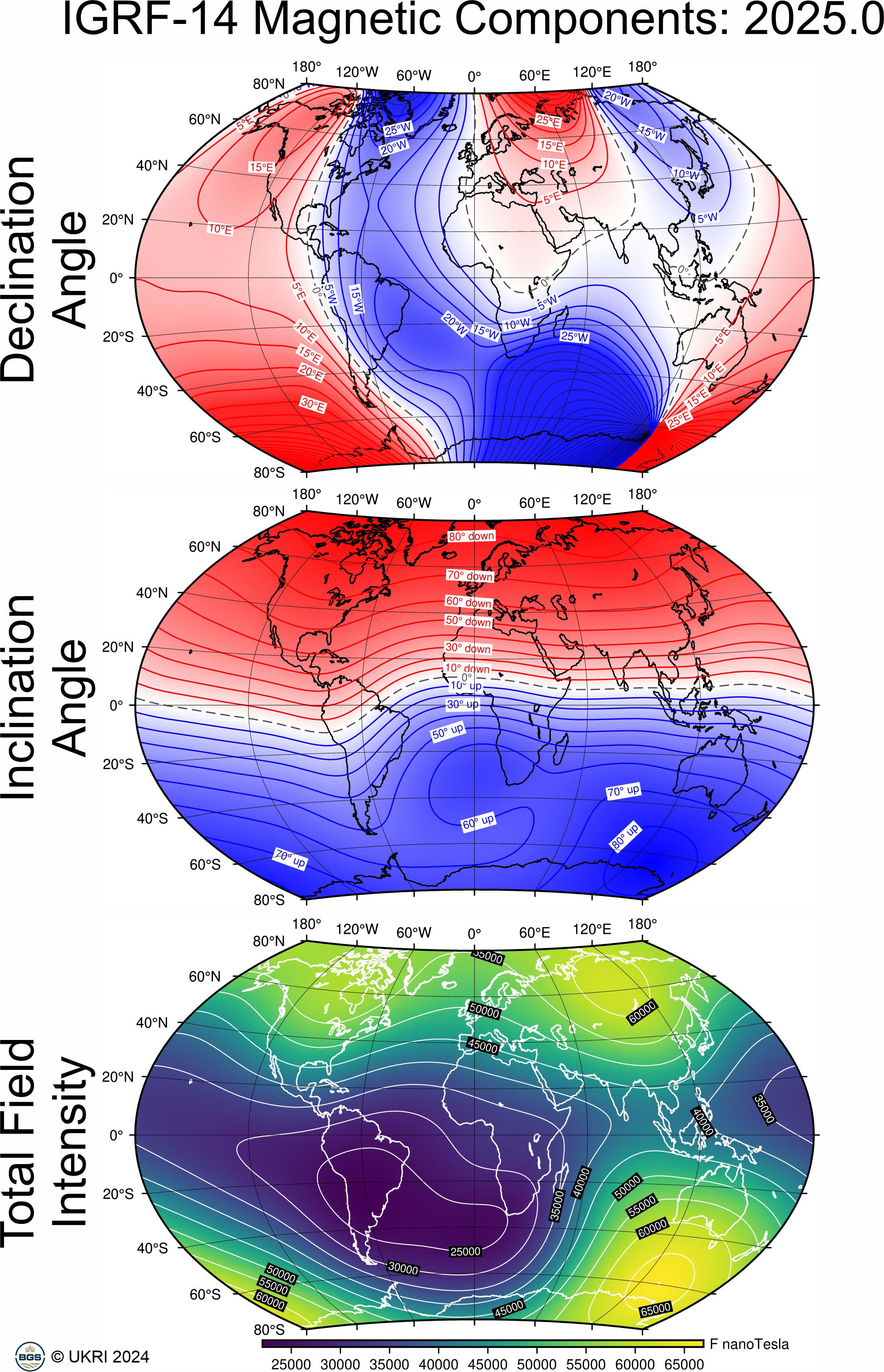
Maps of the three components of the magnetic field at 2025. The panels illustrate the Declination angle (i.e. angle between true and magnetic North), the Inclination (or magnetic dip) and Total Field Intensity from IGRF-14.
Resolving velocity distribution function parameters from observations with significant Poisson statistical uncertainty
By Georgios Nicolaou (Mullard Space Science Laboratory, UCL)
The interpretation of plasma in-situ measurements often involves the application of standard analysis methods to the observations. Some of these methods adopt simplifications that lead to erroneous results. A recently published study led by Georgios Nicolaou uses simulations of plasma measurements and evaluates the statistical errors of plasma parameters determined by applying three different analysis methods to the data. The study shows that two classic fitting techniques that use chi-squared minimization result in significant systematic misestimations of the plasma parameters when applied to samples with credible statistical uncertainty. On the other hand, the application of the Poisson maximum likelihood method to the same data samples always returns the plasma parameters with negligible systematic errors. The authors quantify the expected errors of the examined methods as functions of the statistical significance of the observations. A follow-up study led by Georgios shows that a classic chi-squared minimization method creates artificial correlations to the determined plasma densities and temperatures, which may be misinterpreted as an actual characteristic behaviour of the examined plasma. However, this is not an issue when the Poisson maximum likelihood method is used to analyse the same observations.
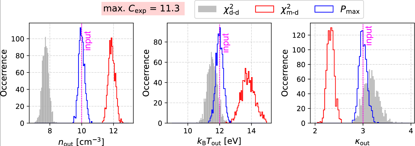
Histograms of plasma bulk parameters determined by applying the three different fit methods to the same measurement samples.
(Left) Plasma density, (middle) temperature, and (right) kappa index, determined by using
Method A: chi-squared minimization with data-driven uncertainty (grey),
Method B: chi-squared minimization with model-driven uncertainty (red), and
Method C: maximum-likelihood method (blue).
The actual plasma parameters (simulation input) are indicated by the vertical magenta line in each panel.
Publications:
Nicolaou, G., Livadiotis, G., Sarlis, N., Ioannou, C. Resolving velocity distribution function parameters from observations with significant Poisson statistical uncertainty, RAS Techniques and Instruments, 2024 3, 874, https://doi.org/10.1093/rasti/rzae059
Nicolaou, G., Livadiotis, G., Ioannou, C. Artificial Polytropic Behavior of Plasmas Determined from the Application of Chi-squared Minimization Analysis to Data with Significant Statistical Uncertainty, The Astrophysical Journal, 2024, 977, 168, 10.3847/1538-4357/ad8f35
Characterising meso-scale ionospheric flow structures
By Gareth Chisham (British Antarctic Survey)
Measuring and understanding ionospheric plasma flow vorticity aids the study of ionospheric plasma transport processes, such as convection and turbulence, which form an important component of magnetosphere to atmosphere space weather models. This plasma flow is dominated by the large-scale convection driven by solar wind-magnetosphere-ionosphere coupling.
This study (https://doi.org/10.1029/2024JA032887) exploits a recently-developed technique that allows the removal of this large-scale component from probability density functions (PDFs) of ionospheric vorticity measured by the Super Dual Auroral Radar Network (SuperDARN). Following this removal, the residual PDFs are symmetric double-sided functions that describe the meso-scale vorticity component that derives from processes below the large scale, such as turbulence. The character of this meso-scale component varies with location in the polar ionosphere, as shown in the figure. The ability to characterise the meso-scale flows in different regions helps to improve our understanding of the meso-scale processes occurring there. Models of ionospheric plasma flow are an important component in larger-scale system models. However, at the present time, these plasma flow models only consider the large-scale convection flow. Understanding, and being able to model, meso-scale ionospheric vorticity will help improve the accuracy of these models.
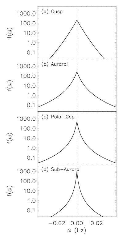
This figure presents schematic representations of the typical probability density functions (PDFs – f(ω))
of meso-scale ionospheric vorticity (ω) that are observed in different regions of the polar ionosphere:
(a) Dayside cusp; (b) Auroral region; (c) Polar cap; (d) Sub-auroral region.
Publication:
Chisham, G., and Freeman, M.P., The spatial variation of large- and meso-scale plasma flow vorticity statistics in the high-latitude ionosphere and implications for ionospheric plasma flow models. J. Geophys. Res., 129, e2024JA032887, 2024.
https://doi.org/10.1029/2024JA032887
Observation of a Fully-formed Forward–Reverse Shock Pair due to the Interaction between Two Coronal Mass Ejections at 0.5 au
By Domenico Trotta (Imperial College London)
The Sun is an active star, responsible for creating a highly dynamic and complex environment, namely the heliosphere. Solar eruptive phenomena are key consequences of such activity, which recently reached the peak of its 11-years cycle, and their study is of paramount importance to understand many unsolved mysteries of how energy is converted in space and astrophysical plasmas [1], as well as to advance our understanding of space weather, for which they are major drivers [2]. Further, novel spacecraft missions, such as Solar Orbiter [3], are opening a novel observational window into such phenomena with revolutionary measurements in the poorly explored inner heliospheric regions close to the Sun.
Solar eruptive phenomena can drive shock waves in the heliosphere (i.e., interplanetary IP shocks), which crucially can be detected in-situ, thus representing the missing link to remote observations of astrophysical systems. Sometimes IP shocks are observed in forward-reverse pairs, propagating away and towards the Sun in the local plasma frame. Forward-reverse shock pairs typically bound compressed plasma regions at solar wind Stream Interaction Regions (SIRs) between slow and fast wind originating from coronal holes [4]. Early observational evidence shows that fully formed forward-reverse shock pairs are very rare in the inner heliosphere, and more commonly observed beyond 1 AU [5]. Conversely, Coronal Mass Ejections (CMEs), the largest eruptive events from the Sun, are routinely found driving forward shocks able to accelerate particles to high energies [6]. Further, interaction between multiple CMEs has been shown as a promising pathway for fast energy conversion in the heliosphere, with a complex range of phenomena being observed in such interaction.
In our study, exploiting the in-situ Solar Orbiter instrument payload, we identified a fully formed forward-reverse shock pair at the unusually short heliocentric distance of 0.5 AU. The observation is shown in Figure 1. We found that such shock pair was not originating from a solar wind SIR, but rather from the interaction between a fast CME interacting with a preceding, slow CME, thereby creating a compression region driving the shock pair due its expansion. This enabled us to study IP shocks in highly unusual parameter regimes (for example the forward shock propagating in CME material). Further, in the interaction region between the two CMEs, a large range of interesting phenomena of energy conversion, such as enhanced rate of magnetic reconnection, has been identified.
We then used remote observations from STEREO-A to identify the two CMEs as they were ejected from the Sun, revealing that the first, slow CME was an extremely faint event. Finally, we used well the radially aligned Wind spacecraft to investigate the fate of such interesting structure, and found that it dissipated at 1 AU, where only a weak forward shock is observed, in stark contrast with SIR-driven shock pairs expected to become stronger with heliocentric distances. Thus, we highlighted how without Solar Orbiter at inner heliocentric distance, such structure would not have been possible to observe and investigate, once again underlining how exploiting multiple heliospheric vantage points is invaluable to advance our understanding of both the Sun-Earth system and remote astrophysical environments.
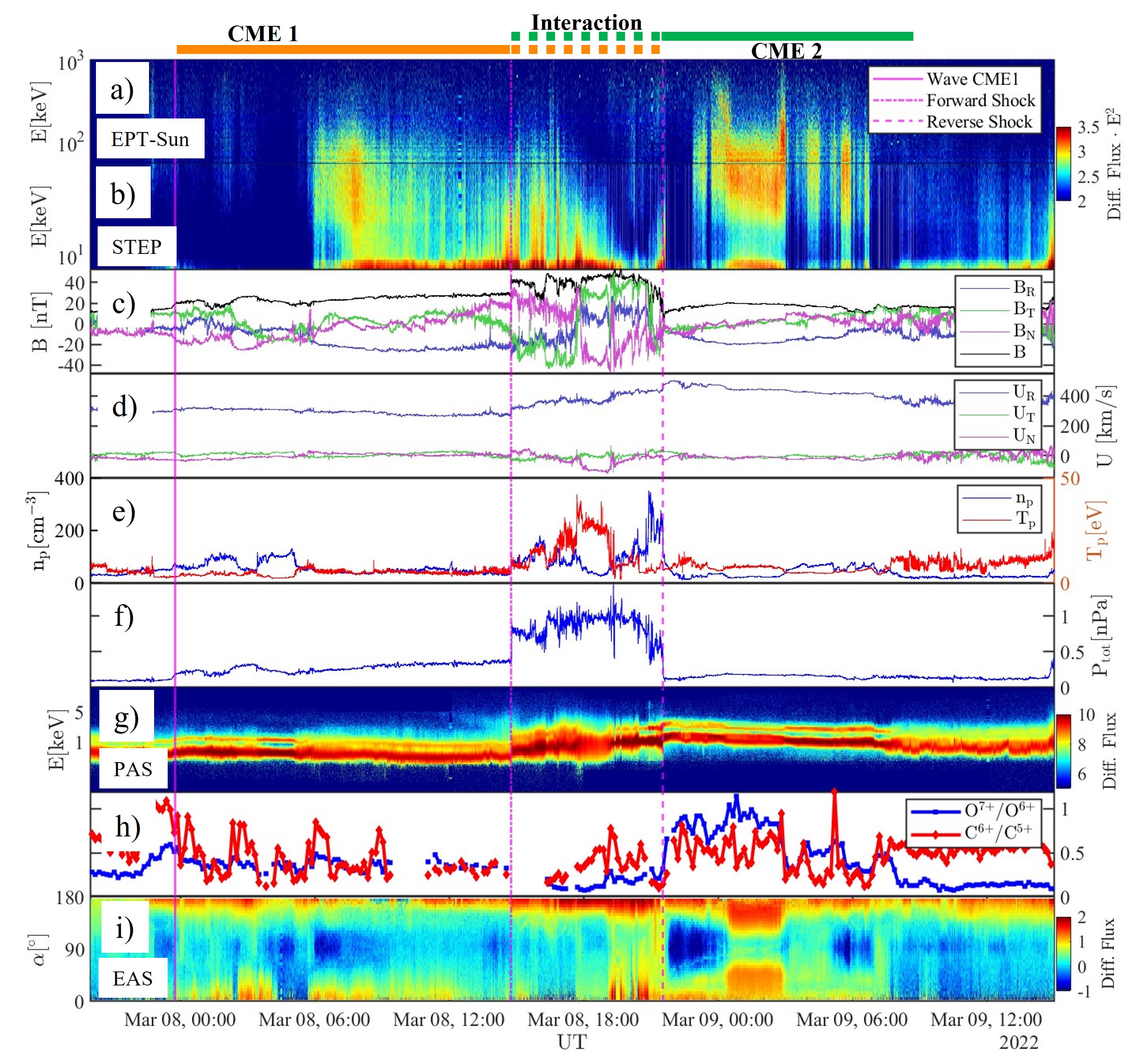
Solar Orbiter direct observation of the forward-reverse shock pair and the interacting CMEs
(full details in the publication).
References:
[1] Rice et al., JGR: Space Physics, 108, 1369 (2003)
[2] Temmer, Liv. Rev. in Sol. Phys., 18, 4 (2021)
[3] Muller et al., A&A, 642, A1 (2020)
[4] Belcher, ApJ, 168, 509 (1971)
[5] Jian et al., Sol. Physics, 239, 337 (2006)
[6] Chen, Liv. Rev. in Sol. Phys., 8, 1 (2011)
See publication for details:
Domenico Trotta et al 2024 ApJL 971 L35
DOI 10.3847/2041-8213/ad68fa
Temperature anisotropy instabilities driven by intermittent velocity shears in the solar wind
By Simon Opie (Mullard Space Science Laboratory, University College London)
Where and under what conditions the transfer of energy between electromagnetic fields and particles takes place in the solar wind remains an open question. In this paper we resolve to find a quantitative and causative link between turbulence in the solar wind and the occurrence of temperature anisotropy in the proton distribution as measured by Solar Orbiter’s Proton Alpha Sensor (PAS) which is part of the Solar Wind Analyser’s (SWA) suite of instruments. We define and derive the radial rate of strain ΓR as a dynamical measure of the driving of temperature anisotropy by bulk plasma motions. Intervals in the data unstable to the oblique firehose and mirror-mode instabilities are on average characterised by high absolute values of ΓR. We attribute this observation to the proposition that temperature anisotropies associated with these kinetic instabilities are the result of strong, intermittent velocity shears in the turbulent solar wind that cause shearing of the frozen-in magnetic field, with a local double-adiabatic impact on the particle distributions.
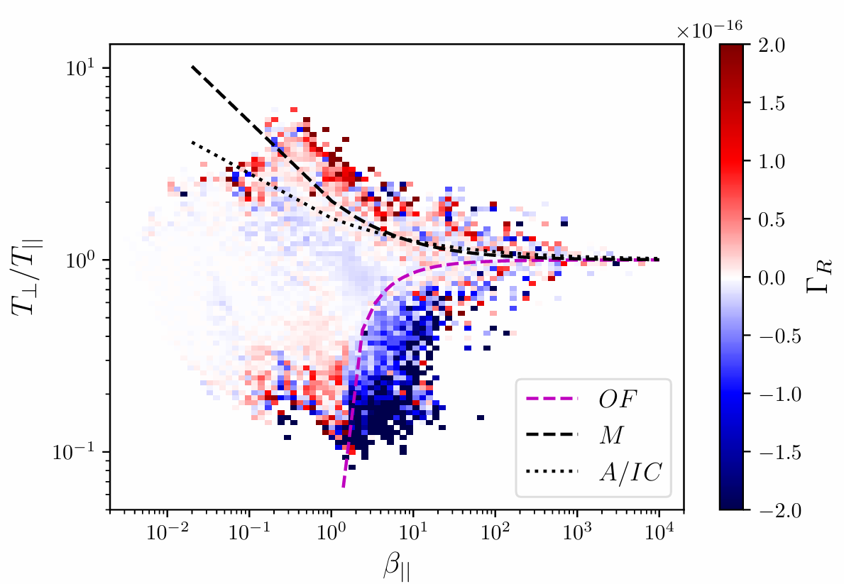
We show the distribution of ΓR as bin averages in T⊥/T∥–β∥ parameter space, where T is the temperature, β is the ratio of plasma pressure to magnetic pressure, and the subscripts represent measurement of the quantity either perpendicular (⊥) or parallel (||) to the magnetic field. We overplot the instability thresholds for the Oblique Firehose (OF), Alfvén/Ion cyclotron (A/IC), and Mirror-mode (M) instabilities. We see that the areas of parameter space beyond the thresholds for the oblique firehose and mirror-mode instabilities are well defined by extreme values in the distribution of ΓR.
See publication for details:
Opie, S., Verscharen, D., Chen, C.H.K., Owen, C.J., Isenberg, P.A., Sorriso-Valvo, L., Franci, L., Matteini, L., 2024. Temperature anisotropy instabilities driven by intermittent velocity shears in the solar wind.
https://doi.org/10.1017/s0022377824001375