MIST
Magnetosphere, Ionosphere and Solar-Terrestrial
Latest articles
- Analysis of Chorus Wave Power on Burst‐Mode Timescales During the Van Allen Probes Era
- Soft X-Ray Emission from Saturn's Magnetosheath II: Solar Wind Driving
- Which Kelvin-Helmholtz waves grow along the spatially-varying magnetopause flanks and why?
- A new declining phase precursor and an early prediction of cycle 26 maximum
- Short-Term Variability of Jupiter's Satellite Footprints as Spotted by JWST
Latest news
Open Letter Ready For Signatories
Protect MIST Science! Sign the MIST Community Open Letter on the STFC funding cuts!
https://sites.google.com/view/uk-mist-community-open-letter
Statement from MIST Council regarding the STFC Funding Situation
Statement from MIST Council regarding the STFC Funding Situation
MIST Council is deeply concerned by the ongoing STFC funding uncertainty and its impact on our community and beyond.
The current combination of prospective delayed and reduced funding, together with already volatile financial situations at universities across the UK, is placing significant strain on research groups. In some cases, institutions may be unable to support researchers through gaps between projects, increasing precarity across the community and adding significant pressure on early-career researchers.
We are concerned that continued uncertainty risks accelerating a brain drain from the UK, as skilled researchers reconsider their future in a system offering limited stability. The loss of expertise at any career stage would have lasting consequences for UK space science.
What is going on?
For those that are unaware of the situation, it is complex and evolving. We suggest the following sources to get up to speed on the current developments.
https://ras.ac.uk/news-and-press/news/proposed-budget-cuts-catastrophe-uk-astronomy
What are we doing about it?
Behind the scenes, MIST Council is actively engaging with relevant parties to understand the scale of the challenge and to identify constructive ways forward.
- We are seeking seasoned members of the community to join MIST Council on a task force to help develop options and represent the needs of our community. If you would like to be involved, please reach out to us via the MIST Council email (This email address is being protected from spambots. You need JavaScript enabled to view it.) by the end of this week (13th February 2026).
- In addition to the task force, we want to provide an open forum for discussion and collective input among all members of the wider MIST community. We are exploring options and will be in touch as soon as possible with further details.
- We believe in working together in the face of the current challenges and we are collaborating with UKSP and others to strive for a fair and positive outcome for all. We are reaching out to members of the SSAP (Solar System Advisory Panel) to explore the hosting of a community town hall meeting, like the one already being organised by the AAP (Astronomy Advisory Panel), to provide an open forum for discussion and collective input.
What can you do to help?
There are several open letters representing people in various career stages that have been made available to sign. We encourage you to read the relevant letter(s) and to sign them if you support them:
- Fellowship Holders: https://advancedfellows-openletter-stfc.github.io/index.html
- Early Career Researchers: https://ecr-openletter-stfc.github.io/
The Royal Astronomical Society are also urging Fellows to lobby their MPs against the cuts, and have included a template letter that can be used to do so:
https://ras.ac.uk/news-and-press/news/ras-fellows-urged-lobby-against-unprecedented-cuts
MIST Council will continue to advocate for transparency, stability, and funding structures that recognise both the long-term nature of our science and the people who deliver it.
We thank you for your continued support in this period of uncertainty.
Please contact This email address is being protected from spambots. You need JavaScript enabled to view it. if you have further suggestions.
MIST Council
![]()
Announcement of New MIST Council 2025
We are very pleased to announce the following members of the community have been elected to MIST Council:
- Gemma Bower (University of Leicester), MIST Councillor
- Tom Elsden (University of St Andrews), MIST Councillor
- Cameron Patterson (Lancaster University), MIST Councillor
- Fiona Ball (University of Southampton), Student Representative
They will begin their terms in July 2025.
We thank outgoing MIST Council members: Maria Walach, Chiara Lazzeri and Emma Woodfield. Andy Smith will remain on council a little longer as a co-opted member to cover Rosie Johnson's maternity leave.
The current composition of Council can be found on our website (https://www.mist.ac.uk/community/mist-council).
Announcement of New MIST Councillors.
We are very pleased to announce the following members of the community have been elected unopposed to MIST Council:
- Rosie Johnson (Aberystwyth University), MIST Councillor
- Matthew Brown (University of Birmingham), MIST Councillor
- Chiara Lazzeri (MSSL, UCL), Student Representative
Rosie, Matthew, and Chiara will begin their terms in July. This will coincide with Jasmine Kaur Sandhu, Beatriz Sanchez-Cano, and Sophie Maguire outgoing as Councillors.
The current composition of Council can be found on our website, and this will be amended in July to reflect this announcement (https://www.mist.ac.uk/community/mist-council).
Nominations are open for MIST Council
We are very pleased to open nominations for MIST Council. There are three positions available (detailed below), and elected candidates would join Georgios Nicolaou, Andy Smith, Maria-Theresia Walach, and Emma Woodfield on Council. The nomination deadline is Friday 31 May.
Council positions open for nomination
2 x MIST Councillor - a three year term (2024 - 2027). Everyone is eligible.
MIST Student Representative - a one year term (2024 - 2025). Only PhD students are eligible. See below for further details.
About being on MIST Council
If you would like to find out more about being on Council and what it can involve, please feel free to email any of us (email contacts below) with any of your informal enquiries! You can also find out more about MIST activities at mist.ac.uk. Two of our outgoing councillors, Beatriz and Sophie, have summarised their experiences being on MIST Council below.
Beatriz Sanchez-Cano (MIST Councillor):
"Being part of the MIST council for the last 3 years has been a great experience personally and professionally, in which I had the opportunity to know better our community and gain a larger perspective of the matters that are important for the MIST science progress in the UK. During this time, I’ve participated in a number of activities and discussions, such as organising the monthly MIST seminars, Autumn MIST meetings, writing A&G articles, and more importantly, being there to support and advise our colleagues in cases of need together with the wonderful council members. MIST is a vibrant and growing community, and the council is a faithful reflection of it."
Sophie Maguire (MIST Student Representative):
"Being the student representative for MIST council has been an amazing experience. I have been part of organizing conferences, chairing sessions, and writing grant applications based on the feedback MIST has received. From a wider perspective, MIST has helped to grow and support my professional networks which in turn, directly benefits my PhD work as well. I would encourage any PhD student to apply for the role of MIST Student Representative and I would be happy to answer any questions or queries you have about the role."
How to nominate
If you would like to stand for election or you are nominating someone else (with their agreement!) please email This email address is being protected from spambots. You need JavaScript enabled to view it. by Friday 31 May. If there is a surplus of nominations for a role, then an online vote will be carried out with the community. Please include the following details in the nomination:
- Name
- Position (Councillor/Student Rep.)
- Nomination Statement (150 words max including a bit about the nominee and focusing on your reasons for nominating. This will be circulated to the community in the event of a vote.)
MIST Council details
- Sophie Maguire, University of Birmingham, Earth's ionosphere - This email address is being protected from spambots. You need JavaScript enabled to view it.
- Georgios Nicolaou, MSSL, solar wind plasma - This email address is being protected from spambots. You need JavaScript enabled to view it.
- Beatriz Sanchez-Cano, University of Leicester, Mars plasma - This email address is being protected from spambots. You need JavaScript enabled to view it.
- Jasmine Kaur Sandhu, University of Leicester, Earth’s inner magnetosphere - This email address is being protected from spambots. You need JavaScript enabled to view it.
- Andy Smith, Northumbria University, Space Weather - This email address is being protected from spambots. You need JavaScript enabled to view it.
- Maria-Theresia Walach, Lancaster University, Earth’s ionosphere - This email address is being protected from spambots. You need JavaScript enabled to view it.
- Emma Woodfield, British Antarctic Survey, radiation belts - This email address is being protected from spambots. You need JavaScript enabled to view it.
- MIST Council email - This email address is being protected from spambots. You need JavaScript enabled to view it.
Nuggets of MIST science, summarising recent papers from the UK MIST community in a bitesize format.
If you would like to submit a nugget, please fill in the following form: https://forms.gle/Pn3mL73kHLn4VEZ66 and we will arrange a slot for you in the schedule. Nuggets should be 100–300 words long and include a figure/animation. Please get in touch!
If you have any issues with the form, please contact This email address is being protected from spambots. You need JavaScript enabled to view it..
Equatorial magnetosonic waves observed by Cluster satellites: The Chirikov resonance overlap criterion
by Homayon Aryan (University of Sheffield)
Numerical codes modelling the evolution of the radiation belts often account for wave-particle interaction with magnetosonic waves. The diffusion coefficients incorporated in these codes are generally estimated based on the results of statistical surveys of the occurrence and amplitude of these waves. These statistical models assume that the spectrum of the magnetosonic waves can be considered as continuous in frequency space, however, this assumption can only be valid if the discrete nature of the waves satisfy the Chirikov resonance overlap criterion.
The Chirikov resonance overlap criteria describes how a particle trajectory can move between two resonances in a chaotic and unpredictable manner when the resonances overlap, such that it is not associated with one particular resonance [Chirikov, 1960]. It can be shown that the Chirikov resonance overlap criterion is fulfilled if the following equation is satisfied:
δθ = (vl / tanθm) / (1 - (ω2/vΩce2))
where θm is the mean angle between the propagation direction and the external magnetic field, δθ is the standard deviation of the wave propagation angles , l is the harmonic number, v=me/mp is the electron to proton mass ratio, and Ωce is the electron gyro-frequency [Artemyev et al., 2015].
Here we use Cluster observations of magnetosonic wave events to determine whether the discrete nature of the waves always satisfy the Chirikov resonance overlap criterion, extending a case study by Walker et al. [2015]. An example of a magnetosonic wave event is shown in panels a-c of the Figure. Panel d shows that the Chirikov overlap criterion is satisfied for this case. However, a statistical analysis shows that most, but not all, discrete magnetosonic emissions satisfy the Chirikov overlap criterion. Therefore, the use of the continuous spectrum, assumed in wave models, may not always be justified. We also find that not all magnetosonic wave events are confined very close to the magnetic equator as it is widely assumed. Approximately 75% of wave events were observed outside 3° and some at much higher latitudes ~21° away from the magnetic equator. This observation is consistent with some past studies that suggested the existence of low-amplitude magnetosonic waves at high latitudes. The results highlight that the assumption of a continuous frequency spectrum could produce erroneous results in numerical modelling of the radiation belts.
For more information please see the paper below:
, , , & ( 2019). Equatorial magnetosonic waves observed by Cluster satellites: The Chirikov resonance overlap criterion. Journal of Geophysical Research: Space Physics, 124. https://doi.org/10.1029/2019JA026680
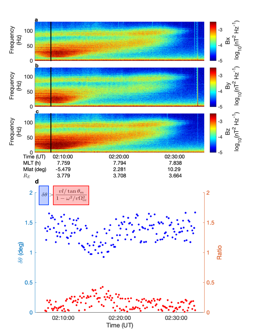
Figure: Observation of a magnetosonic wave event measured by Cluster 2 on 16 November 2006 at around 02:08 to 02:33~UT. The top three panels (a, b, and c) show the dynamic wave spectrogram (Bx, By, and Bz respectively) measured by STAFF search coil magnetometer. Panel d shows the analysis of the Chirikov resonance overlap criterion outlined in equation shown on top-left of the panel. The blue and red dots represent 10~s averaged values of dqand the ratio on the right hand side of equation respectively.
How well can we estimate Pedersen conductance from the THEMIS white-light all-sky cameras?
by Mai Mai Lam (University of Southampton)
The substorm cycle comprises the loading and explosive release of magnetic energy into the Earth system, causing complex and brilliant auroral light displays as large as a continent. Within one substorm, over 50% of the total solar wind energy input to the Earth system is estimated to be converted to Joule heating of the atmosphere.Such Joule heating is highly variable, and difficult to measure for individual substorms. One quantity that we need to measure in order to calculate the Joule heating is the distribution of Pedersen conductance. Ideally this should be done across the very large range of latitudes and local times that substorms expand into. Pedersen conductance can be examined with high accuracy by exploiting ground-based incoherent scatter radar data, but only on the scale of a few kilometres.
The THEMIS all-sky imagers form a network of nonfiltered cameras that spans North America. Previous results have shown that the optical intensity of a single ground camera with a green filter can be used to find a reasonable estimate of Pedersen conductance. Therefore we asked whether THEMIS white-light cameras could measure the conductance as precisely as radars can, but at multiple locations across a continent. We found that the conductance estimated by one THEMIS camera has an uncertainty of 40% compared to the radar estimates on a spatial scale of 10 – 100 km and a timescale of 10 minutes. In addition, our results indicate that the THEMIS camera network could identify regions of high and low Pedersen conductance on even finer spatio-temporal scales. This means we can use the THEMIS network, and its data archive, to learn more about how much substorms heat up the atmosphere and how complicated and changeable this behaviour is.
For more information please see the paper below:
“How well can we estimate Pedersen conductance from the THEMIS white‐light all‐sky cameras?”, M. M. Lam , M. P. Freeman, C. M. Jackman, I. J. Rae, N. M. E. Kalmoni, J. K. Sandhu, C. Forsyth. Journal of Geophysical Research. https://doi.org/10.1029/2018JA026067
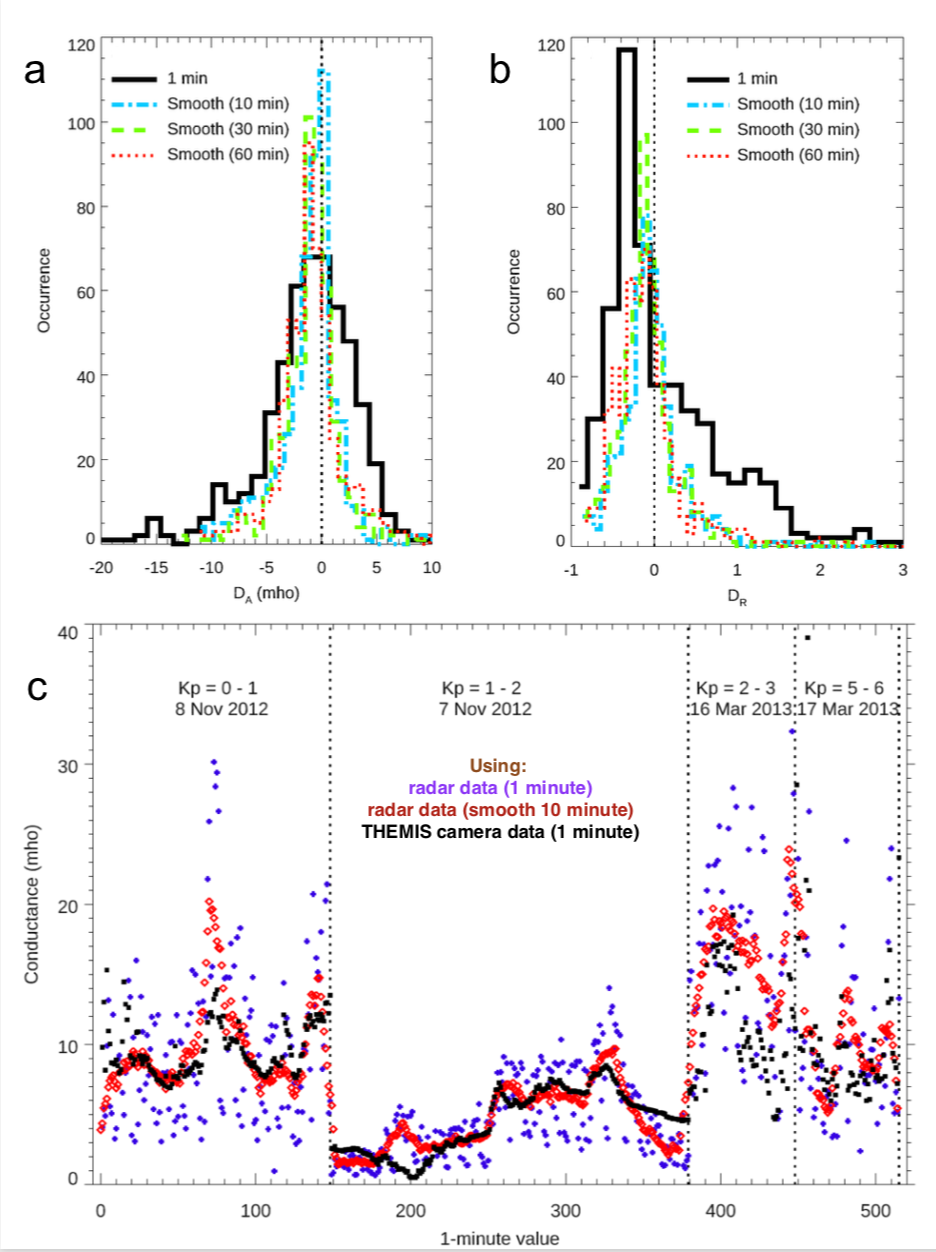
Figure caption: (a) Absolute difference between camera- and radar-derived 1 min Pedersen conductance (black solid) and the effect of different temporal smoothing (coloured broken). (b) As for a, but for the relative difference between camera- and radar-derived Pedersen conductance (normalised to the radar conductance). (c) Comparison of camera-derived and radar-derived Pedersen conductance values for days with different geomagnetic conditions as indicated by Kp: 1 min radar values (blue crosses), 1 min radar values smoothed over 10 min (red diamonds), and 1 min values derived from camera intensity (black squares).
The magnetopause booms like a drum due to impulses
by Martin Archer (Queen Mary University of London)
The abrupt boundary between a magnetosphere and the surrounding plasma, the magnetopause, has long been known to support surface waves which travel down the flanks. However, just like a stone thrown in a pond causes ripples which spread out in all directions, impulses acting on our magnetopause should also cause waves to travel towards the magnetic poles. It had been proposed that the ionosphere might result in a trapping of surface wave energy on the dayside as a standing wave or eigenmode of the magnetopause surface. This mechanism should act as a global source of magnetopause dynamics and ultra-low frequency waves that might then drive radiation belt and auroral interactions.
While many potential impulsive drivers are known, no direct observational evidence of this process had been found to date and searches for indirect evidence had proven inconclusive, casting doubt on the theory. However, Archer et al. (2019) show using all five THEMIS spacecraft during their string-of-pearls phase that this mechanism does in fact occur.
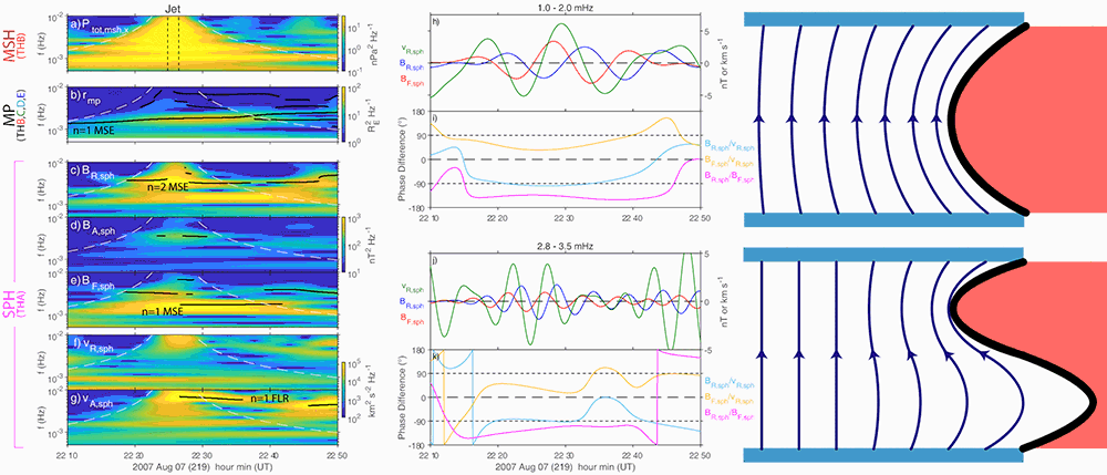
Figure: THEMIS observations and a schematic of the magnetopause standing wave.
They present observations of a rare isolated fast plasma jet striking the magnetopause. This caused motion of the boundary and ultra-low frequency waves within the magnetosphere at well-defined frequencies. Through comparing the observations with the theoretical expectations for several possible mechanisms, they concluded that the jet excited the magnetopause surface eigenmode – like how hitting a drum once reveals the sounds of its normal modes.
Hear the signals as audible sound here: https://www.youtube.com/watch?v=mcG03NBJf-s
For more information please see the paper below:
‘Direct Observations Of A Surface Eigenmode Of The Dayside Magnetopause’. M.O. Archer, H. Hietala, M.D. Hartinger, F. Plaschke, V. Angelopoulos. Nature Communications. | https://doi.org/10.1038/s41467-018-08134-5
Detecting the Resonant Frequency of the Magnetosphere with SuperDARN
by Samuel J. Wharton (University of Leicester)
The Earth’s magnetosphere is constantly being disturbed by ultralow frequency (ULF) waves. These waves transport energy and momentum through the system and can form standing waves on magnetospheric field lines. These standing waves have a resonant frequency which depends on the magnetic field strength and plasma distribution along the field line. The waves result in perturbations in the magnetic field and plasma in the ionosphere. These occur at the resonant frequency and can be directly observed with instruments on the ground. Being able to measure the resonant frequency can provide valuable information about the state of the magnetosphere.
Traditionally, this can be done by applying a cross-phase spectral technique to ground-based magnetometers. It works by finding the frequency where the phase change with latitude is most rapid. This occurs at the local resonant frequency.
The Super Dual Auroral Radar Network (SuperDARN) is a global consortium of 35 radars that observe radio waves backscattered from the ionosphere. The radars detect ULF waves by observing the movements of ionospheric plasma.
For the first time, we have applied the cross-phase technique to SuperDARN. These radars have a much greater spatial resolution and coverage and provide more detailed information than can be achieved with magnetometers alone. In this study, we have used some notable techniques, such as developing a Lomb-Scargle cross-phase technique for uneven data and exploiting an improved fitting procedure Reimer et al. (2018).
We have been able to apply these methods to several examples and validate the results with ground magnetometer estimations. When available, ionospheric heaters can be used to reduce the uncertainty in the backscatter location. However, the majority of SuperDARN data does not have a heater in the field of view and observes ‘natural scatter’. Figure 1 shows an example of the technique applied to natural scatter. The red band in Figure 1e lies at the resonant frequency. Hence, we can measure the resonant frequencies with and without an ionospheric heater.
This study demonstrates that SuperDARN can be used as a tool to monitor resonant frequencies and therefore the plasma distribution of the magnetosphere. This opens up a new application for the SuperDARN radars.
For more information, please see the paper below:
Wharton, S. J., Wright, D. M., Yeoman, T. K., & Reimer, A. S. (2019). Identifying ULF wave eigenfrequencies in SuperDARN backscatter using a Lomb-Scargle cross-phase analysis. Journal of Geophysical Research: Space Physics, 124. https://doi.org/10.1029/2018JA025859
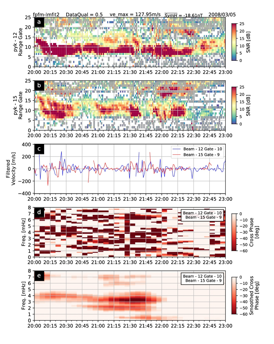
Figure 1: This shows an example of the local resonant frequency being measured by SuperDARN. (a) and (b) show range-time-intensity plots for beams 12 and 15 of the Þykkvibær radar. (c) shows filtered line-of-sight velocities for range gates 10 and 9 on those beams respectively. (d) The cross-phase spectrum for data in (c). (e) The cross-phase spectrum from (d) smoothed.
Current Density in Saturn’s Equatorial Current Sheet: Cassini Magnetometer Observations
by Carley J. Martin (Lancaster University)
Saturn’s rapidly rotating magnetosphere forms an equatorial current sheet that is prone to both periodic (i.e. flapping, breathing [see MIST nugget by Arianna Sorba]) and aperiodic movements (i.e. Martin & Arridge [2017]).
Although the current density of the sheet structure has been discussed by many previous authors, the current density in the middle to outer magnetosphere has not been fully explored. To this end we analysed aperiodic wave movements of Saturn’s current sheet, determined using Cassini’s magnetometer observations. The data were fitted to a deformed current sheet model in order to estimate the magnetic field value just outside of the current sheet, plus the scale height of the current sheet itself. These values were then used to calculate the height integrated current density.
We find a local time asymmetry in the current density, similar to the relationship seen at Jupiter, with a peak in current density of 0.04 A/m at ~ 3 SLT (Saturn Local Time). We then used the divergence of the azimuthal and radial current densities to infer the field-aligned currents that flow out from the equator pre-noon and enter the equator pre-midnight, similar to the Region-2 current at Earth. This current closure could enhance auroral emission in the pre-midnight sector by up to 11 kR.
Overall, the results provide important information into the asymmetries of the current sheet, and the characteristics of the current sheet suggest important field-aligned current systems that shape Saturn’s auroral emissions.
For more information, please see the paper below:
Martin, C. J., & Arridge, C. S. (2019). Current density in Saturn's equatorial current sheet: Cassini magnetometer observations. Journal Geophysical Researcher: Space Physics, 124, 279–292. https://doi.org/10.1029/2018JA025970
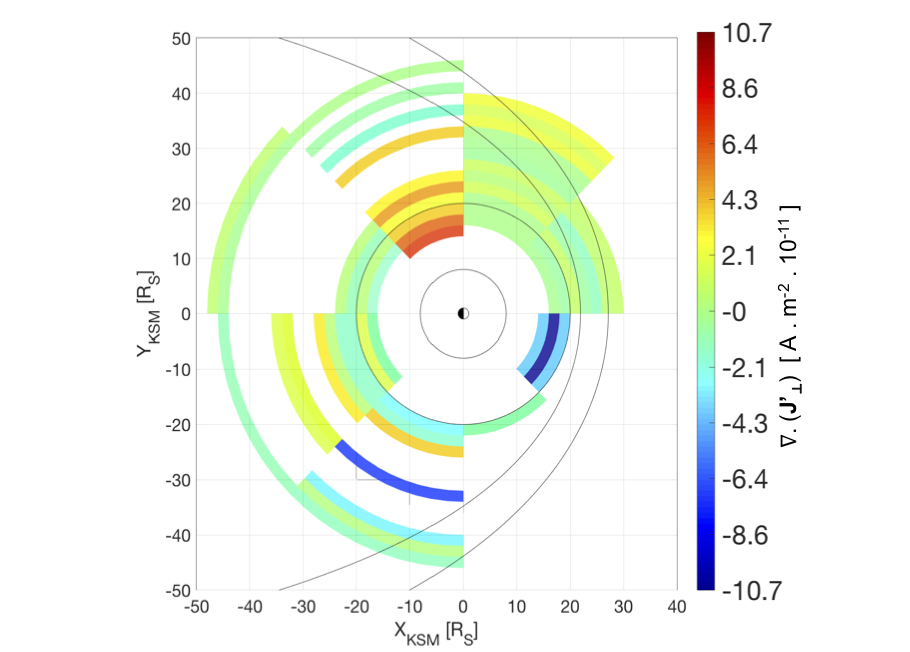
Figure: Divergence of height-integrated perpendicular current density (which infers the field-aligned current density). The coloured blocks show the average value of the divergence projected onto the X-Y plane in KSM (Kronocentric Solar Magnetospheric) coordinates. A range of magnetopause positions is shown using Arridge et at. (2006) along with the orbits of Titan (20 RS) and Rhea (9 RS), all shown in grey.